使用numpy实现批量梯度下降的感知机模型

生成多维高斯分布随机样本

生成多维高斯分布所需要的均值向量和方差矩阵

这里使用numpy中的多变量正太分布随机样本生成函数，按照要求设置均值向量和协方差矩阵。以下设置两个辅助函数，用于指定随机变量维度，生成相应的均值向量和协方差矩阵。

import numpy as np
from numpy.random import multivariate_normal


from math import sqrt

均值向量生成函数

输入：

n：指定随机样本的维度

输出：

m1,m2：正类样本和负类样本的均值向量

def generate_mean_vector(n):
    m1=1/np.sqrt(np.arange(1,n+1))
    m2=-1/np.sqrt(np.arange(1,n+1))
    return m1,m2

协方差矩阵生成函数

输入：

n：指定随机样本的维度

输出：

cov：协方差矩阵，特殊化为对角阵

def generate_cov_matrix(n):
    cov=np.eye(n)
    return cov/n

测试协方差矩阵生成函数

cov=generate_cov_matrix(3)
print(cov)
print(cov.shape)

[[ 0.33333333  0.          0.        ]
 [ 0.          0.33333333  0.        ]
 [ 0.          0.          0.33333333]]
(3, 3)

测试正负样本的均值矩阵生成函数

mean1,mean2=generate_mean_vector(3)
print(mean1)
print(mean2)
len(mean1)

[ 1.          0.70710678  0.57735027]
[-1.         -0.70710678 -0.57735027]





3

生成多维高斯分布的数据点

这里之间调用numpy中的函数

def generate_data(m1,m2,n):
    mean1,mean2=generate_mean_vector(n)
    cov=generate_cov_matrix(n)
    dataSet1=multivariate_normal(mean1,cov,m1)
    dataSet2=multivariate_normal(mean2,cov,m2)
    return dataSet1,dataSet2 

测试数据点生成函数

generate_data(5,5,2)

(array([[ 1.22594293,  0.63712588],
        [ 2.5778577 ,  1.01123791],
        [ 1.16177917,  0.26111813],
        [ 0.27808353,  3.47596707],
        [ 1.07724333,  1.72858977]]), array([[-1.62291142, -1.19754211],
        [-1.0161682 ,  0.9159203 ],
        [-0.98557188, -2.15175781],
        [-0.62078416, -1.11943163],
        [-1.9053243 , -1.36074614]]))

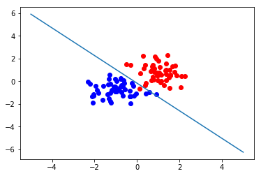
二维数据分布的可视化

from matplotlib import pyplot
class1,class2=generate_data(10,10,2)
class1=np.transpose(class1)
class2=np.transpose(class2)
pyplot.plot(class1[0],class1[1],'ro')
pyplot.plot(class2[0],class2[1],'bo')
pyplot.show()

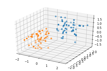
三维数据分布的可视化

#import matplotlib as mpl
#mpl.use('Agg')
from mpl_toolkits.mplot3d import Axes3D
import matplotlib.pyplot as plt
class0,class1=generate_data(50,50,3)
class0=np.transpose(class0)
class1=np.transpose(class1)
fig=plt.figure()
ax=fig.add_subplot(111,projection='3d')
ax.scatter(class0[0],class0[1],class0[2],'ro')
ax.scatter(class1[0],class1[1],class1[2],'ro')
#fig.show()
pyplot.show()

感知机模型类

此模型的接口尽量与sklearn的模型接口保持一致

属性：

lr：learning rate，学习率

dim：样本空间的维度

weight：感知机模型的权重向量，包括偏置（在向量的最后一位）

方法：

init

输入：

lr：感知机模型的学习率

fit

输入：

X_train：训练样本的属性

y_train：训练样本的类别

epochs：算法迭代的最多次数

输出：模型的权重参数

predict

输入：

X：需要预测类别的样本集合

data_extend：布尔型变量，指示输入矩阵X是否经过了扩展预处理

输出：

result：预测结果向量

evaluate

输入：

X_test:测试集的样本属性

y_test：测试集的样本类别

data_extend：测试机样本矩阵是否经过了拓展

输出：

result：一个布尔向量，指示预测是否正确

get_weight

输出：

weight:模型的权重

class Perceptron():
    def __init__(self,lr=0.01):
        self.lr=lr
    def fit(self,X_train,y_train,epochs=10):
        #获取样本空间的维度
        self.dim=X_train.shape[1]
        #初始化权重为零，将最后一个权重作为偏置
        self.weight=np.zeros((1,self.dim+1))
        #拓展样本的维度，将偏置作为权重统一处理
        X_train=np.hstack((X_train,np.ones((X_train.shape[0],1))))
        epoch=0
        while epoch < epochs:
            epoch+=1
            isCorrect=self.evaluate(X_train,y_train,data_extend=True)
            #完全分类正确则停止迭代
            if np.sum(isCorrect)==isCorrect.shape[0]:
                break
            X_error=X_train[np.logical_not(isCorrect)]
            y_error=y_train[np.logical_not(isCorrect)]
            self.weight=self.weight+self.lr*np.dot(y_error,X_error)
    
    #返回预测结果向量    
    def predict(self,X,data_extend=False):
        if data_extend==False:
            X=np.hstack((X,np.ones((X.shape[0],1))))
        p=np.dot(X,np.transpose(self.weight))
        #注意：在这里p是二维数组，要将其转化为一维的
        p=p.ravel()
        p[p>0]=1;p[p<=0]=-1
        return p
    
    #返回布尔向量，如果预测为真则返回一，否则返回零
    def evaluate(self,X_test,y_test,data_extend=False):
        y_pred=self.predict(X_test,data_extend)
        #注意这里是对应位置相乘(只有相乘的两个向量都为一维数组时才成立)
        result=y_pred*y_test
        return result==1
    
    #返回模型参数，最后一个为偏置
    def getweight(self):
        return self.weight

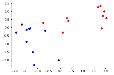
二维样本分类测试与可视化

def test_2d(m1=5,m2=5,epochs=10,lr=0.01):
    X1,X2=generate_data(m1,m2,2)
    X=np.vstack((X1,X2))
    y=np.concatenate(([1]*m1,[-1]*m2))
    model=Perceptron(lr)
    model.fit(X,y,epochs)
    np.transpose(np.matrix([1,2,3]))*3
    
    c1=np.transpose(X1)
    c2=np.transpose(X2)

    pyplot.plot(c1[0],c1[1],'ro')
    pyplot.plot(c2[0],c2[1],'bo')
    w=model.getweight()
    pyplot.plot([-5,5],[-1*w[0,2]/w[0,1]-w[0,0]/w[0,1]*-5,-1*w[0,2]/w[0,1]-w[0,0]/w[0,1]*5])
    pyplot.show()

test_2d(50,50,1000,lr=0.01)

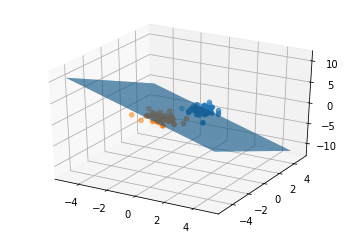
三维样本分类测试与可视化

def test_3d(m1=5,m2=5,epochs=10,lr=0.01):
    X1,X2=generate_data(m1,m2,3)
    X=np.vstack((X1,X2))
    y=np.concatenate(([1]*m1,[-1]*m2))

    model=Perceptron(lr)
    model.fit(X,y,epochs)

    #from matplotlib import pyplot
    c0=np.transpose(X1)
    c1=np.transpose(X2)
  
    from mpl_toolkits.mplot3d import Axes3D
    import matplotlib.pyplot as plt
    
    fig3=plt.figure()
    ax=fig3.add_subplot(111,projection='3d')
    ax.scatter(c0[0],c0[1],c0[2],'ro')
    ax.scatter(c1[0],c1[1],c1[2],'ro')
    w=model.getweight()
    X=np.arange(-5,5,0.05);Y=np.arange(-5,5,0.05)
    X,Y=np.meshgrid(X,Y)
    Z=(w[0,0]*X+w[0,1]*Y+w[0,3])/(-1*w[0,2])
    ax.plot_surface(X,Y,Z,rstride=1,cstride=1)
    ax.set_facecolor('white')
    ax.set_alpha(0.01)
    #fig3.show()
    pyplot.show()

test_3d(50,50,100)