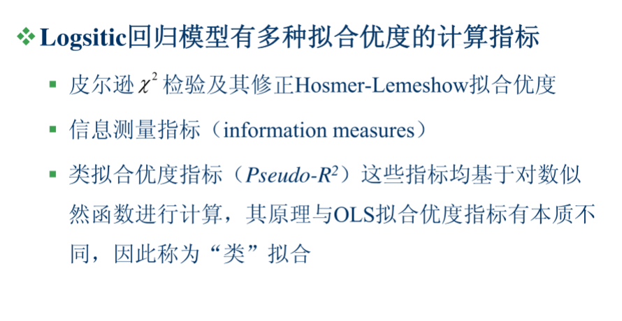
python信用评分卡建模(附代码,博主录制)

预测变量线性检验
当构建一个二元分类器时,很多实践者会立即跳转到逻辑回归,因为它很简单。但是,很多人也忘记了逻辑回归是一种线性模型,预测变量间的非线性交互需要手动编码。回到欺诈检测问题,要获得好的模型性能,像“billing address = shipping address and transaction amount < $50”这种高阶交互特征是必须的。因此,每个人都应该选择适合高阶交互特征的带核SVM或基于树的分类器。
信用评分---是否批准贷款概率---逻辑回归
https://wenku.baidu.com/view/77f741ea5ef7ba0d4a733b6c.html?from=search
概率定义:可能发生事件数量/所有事件数量

odd表示发生概率/不发生概率

odd ratio(两个odd值相比较)
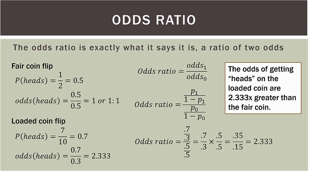
警告:odd和概率是两个不同概念

逻辑回归就是线性的伯努利函数
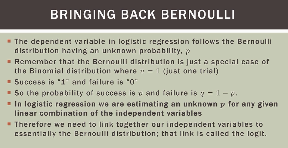
公式用对数函数处理

逻辑回归是计算分类变量概率


二进制数据(分类数据)不呈现正态分布,如果遇到极端的x取值,y预测概率可能偏差较大

对数函数可视化

对数函数里,0-1取值范围在x轴,但我们想要概率到y轴,所以我们去对数函数的反函数


逻辑回归公式


信用得分增加对应得odd概率增加

odd ratio增加可视化图


python脚本实现


# -*- coding: utf-8 -*-

'''
GLM是广义线性模型的一种
Logistic Regression
A logistic regression is an example of a "Generalized Linear Model (GLM)".

The input values are the recorded O-ring data from the space shuttle launches before 1986,
and the fit indicates the likelihood of failure for an O-ring.

Taken from http://www.brightstat.com/index.php?option=com_content&task=view&id=41&Itemid=1&limit=1&limitstart=2
'''


import numpy as np
import matplotlib.pyplot as plt
import pandas as pd
import seaborn as sns

from statsmodels.formula.api import glm
from statsmodels.genmod.families import Binomial

sns.set_context('poster')

def getData():
    '''Get the data '''

    inFile = 'challenger_data.csv'
    data = np.genfromtxt(inFile, skip_header=1, usecols=[1, 2],
                                    missing_values='NA', delimiter=',')
    # Eliminate NaNs
    data = data[~np.isnan(data[:, 1])]

    return data

def prepareForFit(inData):
    ''' Make the temperature-values unique, and count the number of failures and successes.
    Returns a DataFrame'''

    # Create a dataframe, with suitable columns for the fit
    df = pd.DataFrame()
    df['temp'] = np.unique(inData[:,0])
    df['failed'] = 0
    df['ok'] = 0
    df['total'] = 0
    df.index = df.temp.values

    # Count the number of starts and failures
    for ii in range(inData.shape[0]):
        curTemp = inData[ii,0]
        curVal  = inData[ii,1]
        df.loc[curTemp,'total'] += 1
        if curVal == 1:
            df.loc[curTemp, 'failed'] += 1
        else:
            df.loc[curTemp, 'ok'] += 1

    return df

def logistic(x, beta, alpha=0):
    ''' Logistic Function '''
    return 1.0 / (1.0 + np.exp(np.dot(beta, x) + alpha))

def showResults(challenger_data, model):
    ''' Show the original data, and the resulting logit-fit'''

    temperature = challenger_data[:,0]
    failures = challenger_data[:,1]

    # First plot the original data
    plt.figure()
    setFonts()
    sns.set_style('darkgrid')
    np.set_printoptions(precision=3, suppress=True)

    plt.scatter(temperature, failures, s=200, color="k", alpha=0.5)
    plt.yticks([0, 1])
    plt.ylabel("Damage Incident?")
    plt.xlabel("Outside Temperature [F]")
    plt.title("Defects of the Space Shuttle O-Rings vs temperature")
    plt.tight_layout

    # Plot the fit
    x = np.arange(50, 85)
    alpha = model.params[0]
    beta = model.params[1]
    y = logistic(x, beta, alpha)

    plt.hold(True)
    plt.plot(x,y,'r')
    plt.xlim([50, 85])

    outFile = 'ChallengerPlain.png'
    showData(outFile)


if __name__ == '__main__':
    inData = getData()
    dfFit = prepareForFit(inData)

    # fit the model

    # --- >>> START stats <<< ---
    model = glm('ok + failed ~ temp', data=dfFit, family=Binomial()).fit()
    # --- >>> STOP stats <<< ---

    print(model.summary())

    showResults(inData, model)
逻辑回归简化处理-----同盾分数与同盾多头借贷
excel保留两个字段,一个字段是二分类变量,一个字段是数值

同盾分数越高,多头命中概率越高
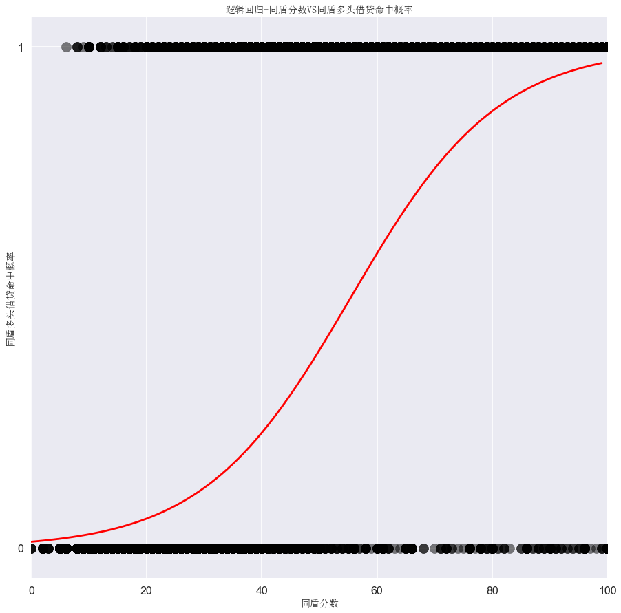
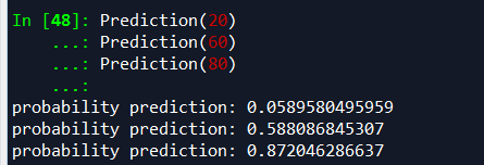
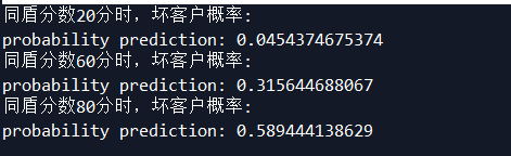
预测,当同盾分数为20,60,80分时,同盾多头借贷命中概率
卡方检验数据偏大,对模型保持谨慎


# -*- coding: utf-8 -*-
"""
Created on Wed Mar  7 10:07:49 2018

@author: Administrator
"""

import csv
import numpy as np
import pandas as pd
from statsmodels.formula.api import glm
from statsmodels.genmod.families import Binomial
import matplotlib.pyplot as plt
import seaborn as sns
#中文字体设置
from matplotlib.font_manager import FontProperties
font=FontProperties(fname=r"c:windowsfontssimsun.ttc",size=14)

#该函数的其他的两个属性"notebook"和"paper"却不能正常显示中文
sns.set_context('poster')

fileName="同盾多头借贷与同盾分数回归分析.csv"
reader = csv.reader(open(fileName))


#获取数据,类型:阵列
def getData():
    '''Get the data '''

    inFile = '同盾多头借贷与同盾分数回归分析.csv'
    data = np.genfromtxt(inFile, skip_header=1, usecols=[0, 1],
                                    missing_values='NA', delimiter=',')
    # Eliminate NaNs 消除NaN数据
    data1 = data[~np.isnan(data[:, 1])]
    return data1


def prepareForFit(inData):
    ''' Make the temperature-values unique, and count the number of failures and successes.
    Returns a DataFrame'''

    # Create a dataframe, with suitable columns for the fit
    df = pd.DataFrame()
    #np.unique返回去重的值
    df['同盾分数'] = np.unique(inData[:,0])
    df['同盾多头借贷命中'] = 0
    df['同盾多头借贷未命中'] = 0
    df['total'] = 0
    df.index = df.同盾分数.values

    # Count the number of starts and failures
    #inData.shape[0] 表示数据多少
    for ii in range(inData.shape[0]):
        #获取第一个值的温度
        curTemp = inData[ii,0]
        #获取第一个值的值,是否发生故障
        curVal  = inData[ii,1]
        df.loc[curTemp,'total'] += 1
        if curVal == 1:
            df.loc[curTemp, '同盾多头借贷命中'] += 1
        else:
            df.loc[curTemp, '同盾多头借贷未命中'] += 1
    return df


#逻辑回归公式
def logistic(x, beta, alpha=0):
    ''' Logistic Function '''
    #点积,比如np.dot([1,2,3],[4,5,6]) = 1*4 + 2*5 + 3*6 = 32
    return 1.0 / (1.0 + np.exp(np.dot(beta, x) + alpha))


#不太懂
def setFonts(*options):
        return
#绘图
def Plot(data,alpha,beta,picName):
    #阵列,数值
    array_values = data[:,0]
    #阵列,二分类型
    array_type = data[:,1]

    plt.figure(figsize=(10,10))
    setFonts()
    #改变指定主题的风格参数
    sns.set_style('darkgrid')
    #numpy输出精度局部控制
    np.set_printoptions(precision=3, suppress=True)
    plt.scatter(array_values, array_type, s=200, color="k", alpha=0.5)
    #获x轴列表值,同盾分数
    list_values = [row[0] for row in inData]
    list_values = [int(i) for i in list_values]
    #获取列表最大值和最小值
    max_value=max(list_values)
    print("max_value:",max_value)
    min_value=min(list_values)
    print("min_value:",min_value)
    #最大值和最小值留有多余空间
    x = np.arange(min_value, max_value+1)
    y = logistic(x, beta, alpha)
    print("test")
    plt.hold(True)
    plt.plot(x,y,'r')
    #设置y轴坐标刻度
    plt.yticks([0, 1])
    #plt.xlim()返回当前的X轴绘图范围
    plt.xlim([min_value,max_value])
    outFile = picName
    plt.ylabel("同盾多头借贷命中概率",fontproperties=font)
    plt.xlabel("同盾分数",fontproperties=font)
    plt.title("逻辑回归-同盾分数VS同盾多头借贷命中概率",fontproperties=font)
    #产生方格
    plt.hold(True)
    #图像外部边缘的调整
    plt.tight_layout
    plt.show(outFile)


#用于预测逻辑回归概率
def Prediction(x):
    y = logistic(x, beta, alpha)
    print("probability prediction:",y)
'''
Prediction(80)
probability prediction: 0.872046286637

Prediction(100)
probability prediction: 0.970179520648

'''

#获取数据
inData = getData()
#得到频率计算后的数据
dfFit = prepareForFit(inData)
#Generalized Linear Model 建立二项式模型
model = glm('同盾多头借贷未命中 +同盾多头借贷命中 ~ 同盾分数', data=dfFit, family=Binomial()).fit()
print(model.summary())
chi2=model.pearson_chi2
'''Out[37]: 46.893438309853522  分数越小,p值越大,H0成立,模型越好'''
print("the chi2 is smaller,the model is better")

alpha = model.params[0]
beta = model.params[1]

Plot(inData,alpha,beta,"logiscti regression")

#测试
Prediction(20)
Prediction(60)
Prediction(80)
逻辑回归参数解读
http://www.doc88.com/p-5876372494494.html
参数解读


4.正则化
在实际应用中,为了防止过拟合,使得模型具有较强的泛化能力,往往还需要在目标函数中加入正则项。在逻辑回归的实际应用中,L1正则应用较为广泛,原因是在面临诸如广告系统等实际应用的场景,特征的维度往往达到百万级甚至上亿,而L1正则会产生稀疏模型,在避免过拟合的同时起到了特征选择的作用。工业界一般采用更快的L-BFGS算法求解。关于L1正则逻辑回归和逻辑回归在广告系统中的实际应用可以参考 这里 。
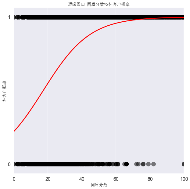
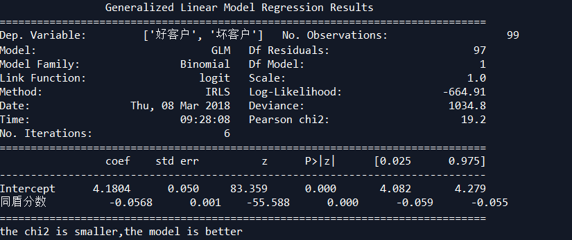
逻辑回归检验好坏客户标签
规则标签,逻辑回归不显著,表明坏客户标签少了
平台B4拒绝,逻辑回归过于显著,表明坏客户标签过多
B4规则
数据保存为CSV逗号格式,CSV utf8格式会报错,而且会丢失数据

# -*- coding: utf-8 -*-
"""
Created on Fri Jul 21 09:28:25 2017
@author: toby
CSV数据结构,第一列为数值,第二列为二分类型
"""
import csv
import numpy as np
import pandas as pd
from statsmodels.formula.api import glm
from statsmodels.genmod.families import Binomial
import matplotlib.pyplot as plt
import seaborn as sns
#中文字体设置
from matplotlib.font_manager import FontProperties
font=FontProperties(fname=r"c:windowsfontssimsun.ttc",size=14)
#该函数的其他的两个属性"notebook"和"paper"却不能正常显示中文
sns.set_context('poster')
fileName="同盾分数与好坏客户_平台拒绝.csv"
reader = csv.reader(open(fileName))
#获取数据,类型:阵列
def getData():
'''Get the data '''
data = np.genfromtxt(fileName, skip_header=1, usecols=[0, 1],
missing_values='NA', delimiter=',')
# Eliminate NaNs 消除NaN数据
data1 = data[~np.isnan(data[:, 1])]
return data1
def prepareForFit(inData):
''' Make the temperature-values unique, and count the number of failures and successes.
Returns a DataFrame'''
# Create a dataframe, with suitable columns for the fit
df = pd.DataFrame()
#np.unique返回去重的值
df['同盾分数'] = np.unique(inData[:,0])
df['坏客户'] = 0
df['好客户'] = 0
df['total'] = 0
df.index = df.同盾分数.values
# Count the number of starts and failures
#inData.shape[0] 表示数据多少
for ii in range(inData.shape[0]):
#获取第一个值的温度
curTemp = inData[ii,0]
#获取第一个值的值,是否发生故障
curVal = inData[ii,1]
df.loc[curTemp,'total'] += 1
if curVal == 1:
df.loc[curTemp, '坏客户'] += 1
else:
df.loc[curTemp, '好客户'] += 1
return df
#逻辑回归公式
def logistic(x, beta, alpha=0):
''' Logistic Function '''
#点积,比如np.dot([1,2,3],[4,5,6]) = 1*4 + 2*5 + 3*6 = 32
return 1.0 / (1.0 + np.exp(np.dot(beta, x) + alpha))
#不太懂
def setFonts(*options):
return
#绘图
def Plot(data,alpha,beta,picName):
#阵列,数值
array_values = data[:,0]
#阵列,二分类型
array_type = data[:,1]
plt.figure(figsize=(10,10))
setFonts()
#改变指定主题的风格参数
sns.set_style('darkgrid')
#numpy输出精度局部控制
np.set_printoptions(precision=3, suppress=True)
plt.scatter(array_values, array_type, s=200, color="k", alpha=0.5)
#获x轴列表值,同盾分数
list_values = [row[0] for row in inData]
list_values = [int(i) for i in list_values]
#获取列表最大值和最小值
max_value=max(list_values)
print("max_value:",max_value)
min_value=min(list_values)
print("min_value:",min_value)
#最大值和最小值留有多余空间
x = np.arange(min_value, max_value+1)
y = logistic(x, beta, alpha)
plt.hold(True)
plt.plot(x,y,'r')
#设置y轴坐标刻度
plt.yticks([0, 1])
#plt.xlim()返回当前的X轴绘图范围
plt.xlim([min_value,max_value])
outFile = picName
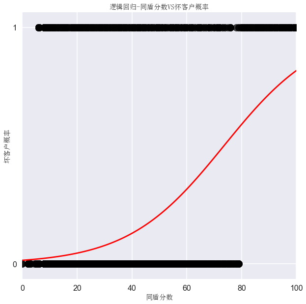
plt.ylabel("坏客户概率",fontproperties=font)
plt.xlabel("同盾分数",fontproperties=font)
plt.title("逻辑回归-同盾分数VS怀客户概率",fontproperties=font)
#产生方格
plt.hold(True)
#图像外部边缘的调整
plt.tight_layout
plt.show(outFile)
#用于预测逻辑回归概率
def Prediction(x):
y = logistic(x, beta, alpha)
print("probability prediction:",y)
'''
Prediction(80)
probability prediction: 0.872046286637
Prediction(100)
probability prediction: 0.970179520648
'''
#获取数据
inData = getData()
#得到频率计算后的数据
dfFit = prepareForFit(inData)
#Generalized Linear Model 建立二项式模型
model = glm('好客户 +坏客户 ~ 同盾分数', data=dfFit, family=Binomial()).fit()
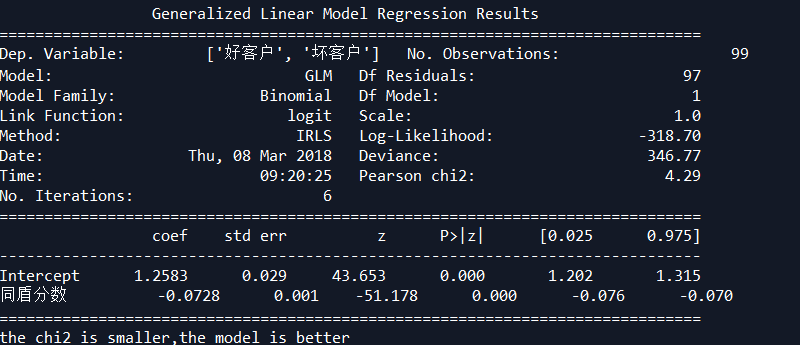
print(model.summary())
chi2=model.pearson_chi2
'''Out[37]: 46.893438309853522 分数越小,p值越大,H0成立,模型越好'''
print("the chi2 is smaller,the model is better")
alpha = model.params[0]
beta = model.params[1]
Plot(inData,alpha,beta,"logiscti regression")
#测试
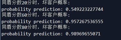
print("同盾分数20分时,坏客户概率:")
Prediction(20)
print("同盾分数60分时,坏客户概率:")
Prediction(60)
print("同盾分数80分时,坏客户概率:")
Prediction(80)
规则标签,逻辑回归不显著,表明坏客户标签少了
逻辑回归评分卡
在建立评分卡模型时,我们经常会使用逻辑回归来对数据进行建模。但在用逻辑回归进行预测时,逻辑回归返回的是一个概率值,并不是评分卡分数。下面为大家介绍如何将模型结果转换为标准评分卡,具体步骤如下:
dvars = {}
scores = {}
df = pd.read_excel("german.xlsx")
df_of_woe = calculate_woe(df)  # 计算woe
df_of_woe.to_excel("german_woe.xlsx")  # 将得到的woe储存
df_of_woe = pd.read_excel("german_woe.xlsx")
iv_list = calculate_iv(df_of_woe)
df_after_iv = filt_by_iv(df_of_woe, 'number', 20)  # 根据iv值选取留下的变量
df_after_pear = remove_pear(df_after_iv, iv_list, 0.1)  # 根据pearson相关系数去除线性相关性较高的变量
df_after_vif = remove_vif(df_of_woe, df_after_pear, 0, 5)  # 根据vif剔除变量,最少剩20个######
logitres, var_list = logitreg(df_after_vif, 0, ks=True)
# joblib.dump(logitres, 'logitres.pkl')
# logitmodel = joblib.load('logitres.pkl')
# dvars:{'Account Balance': [[1, -0.81809870569494136], [2, -0.26512918778930789], [4, 1.1762632228981755]], 'Duration of Credit (month)': [[4, 0.49062291644847106], [18, -0.10423628844554551], [33, -0.76632879785353658]], 'Payment Status of Previous Credit': [[0, -1.2340708354832155], [2, -0.088318616977396236], [3, 0.50972611843257376]], 'Purpose': [[0, 0.077650934230066068], [5, -0.30830135965451672]], 'Credit Amount': [[250, 0.20782931634116719], [3832, -0.33647223662121289], [8858, -1.0624092400041492]], 'Value Savings/Stocks': [[1, -0.27135784446283229], [2, 0.14183019543921782], [4, 0.77780616879129605]], 'Length of current employment': [[1, -0.43113746316229135], [3, -0.032103245384417431], [4, 0.29871666717548989]], 'Instalment per cent': [[1, 0.1904727690246609], [3, 0.064538521137571164], [4, -0.15730028873015464]], 'Sex & Marital Status': [[1, -0.26469255422708216], [3, 0.16164135155641582]], 'Guarantors': [[1, -0.027973852042406294], [3, 0.58778666490211906]], 'Duration in Current address': [[1, -0.017335212001545787], [3, 0.013594092097163191]], 'Most valuable available asset': [[1, 0.46103495926297511], [2, -0.028573372444056114], [3, -0.21829480143299645]], 'Age (years)': [[19, -0.062035390919452635], [41, 0.17435338714477774]], 'Concurrent Credits': [[1, -0.4836298809575007], [2, -0.45953232937844019], [3, 0.12117862465752169]], 'Type of apartment': [[1, -0.40444522020741891], [2, 0.096438848095699109]], 'No of Credits at this Bank': [[1, -0.074877498932750475], [2, 0.1157104960544109], [3, 0.33135713595444244]], 'Occupation': [[1, 0.078471615441495099], [3, 0.022780028331819906], [4, -0.20441251460814672]], 'No of dependents': [[1, -0.0028161099996421362], [2, 0.015408625352845061]], 'Telephone': [[1, -0.064691321198988669], [2, 0.098637588071948196]], 'Foreign Worker': [[1, -0.034867268795640227], [2, 1.262915339959386]]}
x = df.iloc[2:3, 1:]  # 从原始数据集中选取一个观测
print("x for test:", x)  # 打印出来看一眼
x_score = cal_score(logitres, x, dvars, q=600, p=30)  # 得到这个x对应的预测值(01之间)以及得分。
# 默认概率为0.5时为600分,p/1-p每翻一倍多30分
print("x_score:", x_score)
credit_score = (get_score(scores, 30))  # 得到每个变量在不同区间时对应的分数
print("credit score list:", credit_score)
import numpy as np
import pandas as pd
from sklearn.cluster import KMeans
from statsmodels.stats.outliers_influence import variance_inflation_factor
import statsmodels.api as sm
from sklearn.model_selection import train_test_split
import warnings
import matplotlib.pyplot as plt
from sklearn.externals import joblib
from sklearn.metrics import accuracy_score
warnings.filterwarnings("ignore")
def woe_more(item, df, df_woe):
xitem = np.array(df[item])
y = df.loc[:, 'target']
y = np.array(y)
x = []
for k in xitem:
x.append([k])
leastentro = 100
tt_bad = sum(y)
tt_good = len(y) - sum(y)
l = []
for m in range(10):
y_pred = KMeans(n_clusters=4, random_state=m).fit_predict(x)
a = [[[], []], [[], []], [[], []], [[], []]] # 第一项为所有值,第二项为违约情况
for i in range(len(y_pred)):
a[y_pred[i]][0].append(x[i][0])
a[y_pred[i]][1].append(y[i])
a = sorted(a, key=lambda x: sum(x[0]) / len(x[0]))
if sum(a[0][1]) / len(a[0][1]) >= sum(a[1][1]) / len(a[1][1]) >= sum(a[2][1]) / len(a[2][1]) >= sum(a[3][1])
/ len(a[3][1]) or sum(a[0][1]) / len(a[0][1]) <= sum(a[1][1]) / len(a[1][1])
<= sum(a[2][1]) / len(a[2][1]) <= sum(a[3][1]) / len(a[3][1]):
entro = 0
for j in a:
entro = entro + (- (len(j[1]) - sum(j[1])) / len(j[1]) * np.log((len(j[1]) - sum(j[1]))
/ len(j[1])) - sum(
j[1]) / len(j[1]) * np.log(sum(j[1])) / len(j[1]))
if entro < leastentro:
leastentro = entro
l = []
for k in a:
l.append([min(k[0]), max(k[0]), np.log((sum(k[1]) / (len(k[1]) - sum(k[1]))) / (tt_bad / tt_good)),
sum(k[1]) / len(k[1])])
# print (sum(k[1]),len(k[1]))
for m in range(10):
y_pred = KMeans(n_clusters=5, random_state=m).fit_predict(x)
a = [[[], []], [[], []], [[], []], [[], []], [[], []]] # 第一项为所有值,第二项为违约情况
for i in range(len(y_pred)):
a[y_pred[i]][0].append(x[i][0])
a[y_pred[i]][1].append(y[i])
a = sorted(a, key=lambda x: sum(x[0]) / len(x[0]))
if sum(a[0][1]) / len(a[0][1]) >= sum(a[1][1]) / len(a[1][1]) >= sum(a[2][1]) / len(a[2][1]) >= sum(a[3][1])
/ len(a[3][1]) >= sum(a[4][1]) / len(a[4][1]) or sum(a[0][1]) / len(a[0][1]) <= sum(a[1][1]) / len(
a[1][1])
<= sum(a[2][1]) / len(a[2][1]) <= sum(a[3][1]) / len(a[3][1]) <= sum(a[4][1]) / len(a[4][1]):
entro = 0
for k in a:
entro = entro + (- (len(k[1]) - sum(k[1])) / len(k[1]) * np.log((len(k[1]) - sum(k[1]))
/ len(k[1])) - sum(
k[1]) / len(k[1]) * np.log(sum(k[1])) / len(k[1]))
if entro < leastentro:
leastentro = entro
l = []
for k in a:
l.append([min(k[0]), max(k[0]), np.log((sum(k[1]) / (len(k[1]) - sum(k[1]))) / (tt_bad / tt_good)),
sum(k[1]) / len(k[1])])
# print (sum(k[1]),len(k[1]))
if len(l) == 0:
return 0
else:
dvars[item] = []
scores[item] = []
df_woe[item] = [0.0] * len(y_pred)
print('
', "Variable:", item, ": has ", len(l), "categories")
for m in l:
print("span=", [m[0], m[1]], ": WOE=", m[2], "; default rate=", m[3])
dvars[item].append([m[0], m[2]])
scores[item].append([[m[0], m[1]], m[2]])
for i in range(len(y_pred)):
if m[0] <= x[i] <= m[1]:
df_woe[item][i] = float(m[2])
return 1
def woe3(y_pred, item, df, df_woe):
total_bad = sum(df['target'])
total_good = len(df['target']) - total_bad
woe = []
for i in range(3): # 因分成3类,故是3
good, bad = 0, 0 # 每个变量未响应数和未响应数
for j in range(len(y_pred)):
if y_pred[j] == i:
if df['target'][j] == 0:
good = good + 1
else:
bad = bad + 1
if bad == 0:
bad = 1
if good == 0:
good = 1 # 若一个响应/不响应的也没有,就令其有一个,为避免0和inf。大数据下基本不会出现这种情况
woe.append((i, np.log((bad / good) / (total_bad / total_good))))
df_woe[item] = [0.0] * len(y_pred)
for i in range(len(y_pred)):
for w in woe:
if w[0] == y_pred[i]:
df_woe[item][i] = float(w[1])
return woe
def woe2(x_pred, item, df, df_woe):
total_bad = sum(df['target'])
total_good = len(df['target']) - total_bad
X = np.array(df[item])
y_pred = KMeans(n_clusters=2, random_state=1).fit_predict(x_pred) # 用聚类算法按变量位置分好类。已经不需要原始变量了
woe = []
judge = []
for i in range(2):
good, bad = 0, 0 # 每个变量未响应数和响应数
for j in range(len(y_pred)):
if y_pred[j] == i:
if df['target'][j] == 0:
good = good + 1
else:
bad = bad + 1
judge.append([i, bad / (bad + good)])
if bad == 0:
bad = 1
if good == 0:
good = 1 # 若一个响应/不响应的也没有,就令其有一个,为避免0和inf。大数据下基本不会出现这种情况
woe.append((i, np.log((bad / good) / (total_bad / total_good))))
j0, j1 = [], []
for k in range(len(y_pred)):
if y_pred[k] == 0: j0.append(X[k])
if y_pred[k] == 1: j1.append(X[k])
jml = [[np.min(j0), np.max(j0)], [np.min(j1), np.max(j1)]]
for l in range(2):
judge[l].append(jml[l])
judge = sorted(judge, key=lambda x: x[2])
if judge[1][1] - judge[0][1] > 0: # 违约率升序,则woe也升序
woe = sorted(woe, key=lambda x: x[1])
else:
woe = sorted(woe, key=lambda x: x[1], reverse=True)
dvars[item] = []
scores[item] = []
for i in range(2):
# print("span=", judge[i][2], ": WOE=", woe[i][1], "; default rate=", judge[i][1])
dvars[item].append([judge[i][2][0], woe[i][1]])
scores[item].append([judge[i][2], woe[i][1]])
df_woe[item] = [0.0] * len(y_pred)
for i in range(len(y_pred)):
for w in woe:
if w[0] == y_pred[i]:
df_woe[item][i] = float(w[1])
def calculate_woe(df):
df_woe = pd.DataFrame() # 构建一个用于存放woe的pd
for item in list(df)[1:]: # 连续型变量,使用聚类算法分为三类
X = np.array(df[item]) # 原始表格中的一列
x_pred = []
for it in X:
x_pred.append([it]) # 为了进行聚类,对这一列进行处理 ########
flag = 0
print(item, len(set(item)))
if len(set(X)) > 4:
res = woe_more(item, df, df_woe)
if res == 1:
continue
flag = 1
if 2 < len(set(X)) and flag == 0:
for num in range(10):
y_pred = KMeans(n_clusters=3, random_state=num).fit_predict(x_pred) # 用聚类算法按变量位置分好类。已经不需要原始变量了
judge = []
for i in range(3): # 因分成3类,故是3 对每一列进行操作
good, bad = 0, 0 # 每个变量响应数和未响应数
for j in range(len(y_pred)): # ypred是那个有012的
if y_pred[j] == i:
if df['target'][j] == 0:
good = good + 1
else:
bad = bad + 1
judge.append([i, bad / (bad + good)])
j0, j1, j2 = [], [], []
for k in range(len(y_pred)):
if y_pred[k] == 0: j0.append(X[k])
if y_pred[k] == 1: j1.append(X[k])
if y_pred[k] == 2: j2.append(X[k])
jml = [[np.min(j0), np.max(j0)], [np.min(j1), np.max(j1)], [np.min(j2), np.max(j2)]]
for l in range(3):
judge[l].append(jml[l])
judge = sorted(judge, key=lambda x: x[2])
if (judge[1][1] - judge[0][1]) * (judge[2][1] - judge[1][1]) >= 0:
woe = woe3(y_pred, item, df, df_woe)
print('
', "Variable:", item, ": has 3 categories")
if judge[1][1] - judge[0][1] > 0: # 违约率升序,则woe也升序
woe = sorted(woe, key=lambda x: x[1])
else:
woe = sorted(woe, key=lambda x: x[1], reverse=True)
dvars[item] = []
scores[item] = []
for i in range(3):
print("span=", judge[i][2], ": WOE=", woe[i][1], "; default rate=", judge[i][1])
dvars[item].append([judge[i][2][0], woe[i][1]])
scores[item].append([judge[i][2], woe[i][1]])
flag = 1
break
if flag == 0:
print('
', "Variable:", item, ": has 2 categories")
woe2(x_pred, item, df, df_woe)
else:
print('
', "Variable:", item, ": must be 2 categories")
woe2(x_pred, item, df, df_woe)
df_woe['target'] = df['target']
tar = df_woe['target']
df_woe.drop(labels=['target'], axis=1, inplace=True)
df_woe.insert(0, 'target', tar)
return (df_woe)
def calculate_iv(df): # 计算iv值,返回一个包含列名及其对应iv值的list
iv = []
tar = df['target']
tt_bad = sum(tar)
tt_good = len(tar) - tt_bad
for item in list(df)[1:]:
x = df[item]
st = set(x)
for woe in st:
s = 0.0
tt = len(df[df[item] == woe]['target'])
bad = sum(df[df[item] == woe]['target'])
good = tt - bad
s = s + float(bad / tt_bad - good / tt_good) * woe # tt_bad=700,tt_good=300,坏:好=7:3
iv.append([item, s])
return sorted(iv, key=lambda x: x[1])
def filt_by_iv(df, method, alpha): # 根据iv值大小筛选可供使用的变量,默认为20个
iv_list = calculate_iv(df)
vars_to_use = []
if method == "thres":
for item in iv_list:
if item[1] > alpha:
vars_to_use.append(item[0])
if method == "number":
for i in range(alpha):
vars_to_use.append(iv_list[-i - 1][0])
vars_to_use.append('target')
vars_to_use.reverse()
print("the list after iv is: ")
print(vars_to_use)
return df[vars_to_use]
def calculate_pear(x, y, thres=0.8):
r = ((np.dot(x - np.mean(x), y - np.mean(y)) / (len(x) - 1)) / np.sqrt((np.cov(x) * np.cov(y)))) # 相关系数
if abs(r) > thres:
return 1
return 0
def remove_pear(df, iv_list, thres=0.8): # 两两比较变量的线性相关性,若pearson相关系数大于thres就将排序靠后的变量剔除,默认thres=0.8
var_set = set(list(df))
length = len(var_set)
signals = [0] * length
ivd = {}
for item in iv_list:
ivd[item[0]] = item[1]
# 若相关性大,就在s这个list中对其做标记
flag_list = list(var_set)
for i in range(length):
for j in range(i + 1, length):
flag = calculate_pear(df.iloc[:, i], df.iloc[:, j], thres)
if flag == 1:
if flag_list[i] in ivd and flag_list[j] in ivd:
if ivd[flag_list[i]] < ivd[flag_list[j]]:
signals[i] = 1
else:
signals[i] = 1
# st是所需的集合,要从中移除相关性大的变量
for i in range(length):
j = length - 1 - i
if signals[j] == 1:
var_set.remove(flag_list[j])
print("the list after pearson is:", list(var_set))
return list(var_set) # 返回去除完变量后的list
def remove_vif(df, list_after_pear, list_len=20, thres=5.0):
the_set = set(list_after_pear)
while True:
the_list = list(the_set)
new_score = []
for i in range(1, len(the_list)):
new_df = df.drop([the_list[i]], axis=1)
new_ar = np.array(new_df)
new_score.append([i, variance_inflation_factor(new_ar, 0)])
m = sorted(new_score, key=lambda x: x[1], reverse=True)[0] # [最小的label,最小的数]
score = m[1]
if list_len == 0:
if score < float(thres):
break
if list_len != 0:
if score < float(thres) or len(the_set) < list_len:
break
the_set.remove(the_list[m[0]])
final_list = list(the_set)
df_final = df[final_list]
# print (df_final.head())
tar = df_final.pop('target')
df_final.insert(0, 'target', tar)
print("the list after vif is:", list(df_final))
return df_final
def draw_roc(y_pred, y_test, ks=True):
tprlist = []
fprlist = []
auc = 0
ks_list, m1, m2, ks_value = [], [], [], 0
for i in range(1, 1001):
thres = 1 - i / 1000
yp = []
for item in y_pred:
if item > thres:
yp.append(1)
else:
yp.append(0)
Nobs = len(y_test)
h1 = sum(yp)
t1 = sum(y_test)
fn = int((sum(abs(y_test - yp)) + t1 - h1) / 2)
tp = t1 - fn
fp = h1 - tp
tn = Nobs - h1 - fn
fpr = fp / (fp + tn)
tpr = tp / (tp + fn)
tprlist.append(tpr)
fprlist.append(fpr)
ks_list.append(tpr - fpr)
for i in range(999):
auc = auc + (fprlist[i + 1] - fprlist[i]) * tprlist[i]
print("auc=", auc)
plt.plot(fprlist, tprlist)
plt.show()
if ks:
for i in range(10):
m1.append(tprlist[i * 100])
m2.append(fprlist[i * 100])
ks_value = max(ks_list)
print('ks value=', ks_value)
x1 = range(10)
x_axis = []
for i in x1:
x_axis.append(i / 10)
plt.plot(x_axis, m1)
plt.plot(x_axis, m2)
plt.show()
y_pred01 = []
for item in y_pred:
if item > 0.5:
y_pred01.append(1)
else:
y_pred01.append(0)
print("accuracy score=", accuracy_score(y_pred01, y_test))
def logitreg(df, k=0, ks=True):
x = df
x1, x0 = x[x['target'] == 1], x[x['target'] == 0]
y1, y0 = x1['target'], x0['target']
x1_train, x1_test, y1_train, y1_test = train_test_split(x1, y1, random_state=k)
x0_train, x0_test, y0_train, y0_test = train_test_split(x0, y0, random_state=k)
x_train, x_test, y_train, y_test = pd.concat([x0_train, x1_train]), pd.concat([x0_test, x1_test]), pd.concat(
[y0_train, y1_train]), pd.concat([y0_test, y1_test])
x_train, x_test = sm.add_constant(x_train.iloc[:, 1:]), sm.add_constant(x_test.iloc[:, 1:])
var = list(x_train)[1:] # 备选list
st = set()
st.add("const")
while True:
pvs = []
for item in var:
if item not in st:
l = list(st) + [item]
xx = x_train[l]
logit_mod = sm.Logit(y_train, xx)
logitres = logit_mod.fit(disp=False)
pvs.append([item, logitres.pvalues[item]])
v = sorted(pvs, key=lambda x: x[1])[0]
if v[1] < 0.05:
st.add(v[0])
else:
break
ltest = list(st)
xtest = x_train[ltest]
test_mod = sm.Logit(y_train, xtest)
testres = test_mod.fit()
for item in st:
if testres.pvalues[item] > 0.05:
st.remove(item)
print("We have removed item:", item)
print("the list to use for logistic regression:", st)
luse = list(st)
vars_to_del = []
for item in dvars:
if item not in luse:
vars_to_del.append(item)
for item in vars_to_del:
dvars.pop(item)
xuse = x_train[luse]
logit_mod = sm.Logit(y_train, xuse)
logit_res = logit_mod.fit()
print(logit_res.summary())
print("the roc and ks of train set is:")
y_pred = np.array(logit_res.predict(x_test[luse]))
draw_roc(y_pred, y_test, ks)
print("the roc and ks of test set is:")
y_ptrain = np.array(logit_res.predict(x_train[luse]))
draw_roc(y_ptrain, y_train, ks)
return logit_res, luse
def cal_score(res, x, dvars, q=600, p=20):
x = x.loc[:, var_list]
params = res.params # 回归得到的参数
const = params['const']
c = pd.DataFrame([1])
for item in var_list:
if item != 'const':
for i in range(1, len(dvars[item])):
if float(x[item]) < dvars[item][i][0]:
c[item] = dvars[item][i - 1][1]
break
if float(x[item]) >= dvars[item][-1][0]:
c[item] = dvars[item][-1][1]
break
c = c.rename(columns={0: "const"})
res = float(logitres.predict(c))
# print("the result of prediction is:", float(logitres.predict(c)))
score = q - p / np.log(2) * np.log((1 - res) / res)
# print("the credit score is:", score)
return (res, score)
def get_score(scores, p=20):
for item in scores:
for k in scores[item]:
k[1] = k[1] * p / np.log(2)
return scores
dvars = {}
scores = {}
df = pd.read_excel("german.xlsx")
df_of_woe = calculate_woe(df) # 计算woe
df_of_woe.to_excel("german_woe.xlsx") # 将得到的woe储存
df_of_woe = pd.read_excel("german_woe.xlsx")
iv_list = calculate_iv(df_of_woe)
df_after_iv = filt_by_iv(df_of_woe, 'number', 20) # 根据iv值选取留下的变量
df_after_pear = remove_pear(df_after_iv, iv_list, 0.1) # 根据pearson相关系数去除线性相关性较高的变量
df_after_vif = remove_vif(df_of_woe, df_after_pear, 0, 5) # 根据vif剔除变量,最少剩20个######
logitres, var_list = logitreg(df_after_vif, 0, ks=True)
# joblib.dump(logitres, 'logitres.pkl')
# logitmodel = joblib.load('logitres.pkl')
# dvars:{'Account Balance': [[1, -0.81809870569494136], [2, -0.26512918778930789], [4, 1.1762632228981755]], 'Duration of Credit (month)': [[4, 0.49062291644847106], [18, -0.10423628844554551], [33, -0.76632879785353658]], 'Payment Status of Previous Credit': [[0, -1.2340708354832155], [2, -0.088318616977396236], [3, 0.50972611843257376]], 'Purpose': [[0, 0.077650934230066068], [5, -0.30830135965451672]], 'Credit Amount': [[250, 0.20782931634116719], [3832, -0.33647223662121289], [8858, -1.0624092400041492]], 'Value Savings/Stocks': [[1, -0.27135784446283229], [2, 0.14183019543921782], [4, 0.77780616879129605]], 'Length of current employment': [[1, -0.43113746316229135], [3, -0.032103245384417431], [4, 0.29871666717548989]], 'Instalment per cent': [[1, 0.1904727690246609], [3, 0.064538521137571164], [4, -0.15730028873015464]], 'Sex & Marital Status': [[1, -0.26469255422708216], [3, 0.16164135155641582]], 'Guarantors': [[1, -0.027973852042406294], [3, 0.58778666490211906]], 'Duration in Current address': [[1, -0.017335212001545787], [3, 0.013594092097163191]], 'Most valuable available asset': [[1, 0.46103495926297511], [2, -0.028573372444056114], [3, -0.21829480143299645]], 'Age (years)': [[19, -0.062035390919452635], [41, 0.17435338714477774]], 'Concurrent Credits': [[1, -0.4836298809575007], [2, -0.45953232937844019], [3, 0.12117862465752169]], 'Type of apartment': [[1, -0.40444522020741891], [2, 0.096438848095699109]], 'No of Credits at this Bank': [[1, -0.074877498932750475], [2, 0.1157104960544109], [3, 0.33135713595444244]], 'Occupation': [[1, 0.078471615441495099], [3, 0.022780028331819906], [4, -0.20441251460814672]], 'No of dependents': [[1, -0.0028161099996421362], [2, 0.015408625352845061]], 'Telephone': [[1, -0.064691321198988669], [2, 0.098637588071948196]], 'Foreign Worker': [[1, -0.034867268795640227], [2, 1.262915339959386]]}
x = df.iloc[2:3, 1:] # 从原始数据集中选取一个观测
print("x for test:", x) # 打印出来看一眼
x_score = cal_score(logitres, x, dvars, q=600, p=30) # 得到这个x对应的预测值(01之间)以及得分。
# 默认概率为0.5时为600分,p/1-p每翻一倍多30分
print("x_score:", x_score)
credit_score = (get_score(scores, 30)) # 得到每个变量在不同区间时对应的分数
print("credit score list:", credit_score)
def get_q(df):
s0 = []
s1 = []
q = []
for i in range(len(df)):
x = df.iloc[i:i + 1, :]
y = int(x['target'])
x = x.iloc[:, 1:]
score1 = cal_score(logitres, x, dvars, q=600, p=30)
if y == 1:
s1.append(score1)
q.append([score1[0], score1[1], 1])
if y == 0:
s0.append(score1[1])
q.append([score1[0], score1[1], 0])
return q
def get_graph(q):
ss = []
sum_bad = 0
for item in q:
ss.append(item[1])
sum_bad = sum_bad + item[2]
smin = int(min(ss) - 1)
smax = int(max(ss) + 1)
d = (smax - smin) / 10
sscores, xais, tp, fp, rate = [], [], [], [], []
for i in range(10):
sscores.append(int(smin + i * d))
sscores.append(smax)
g, b = 0, 0
pdf = pd.DataFrame(
columns=["good_count", "bad_count", "total", "default_rate", "total_percent", "inside_good_percent",
"inside_bad_percent", "cum_bad", "cum_good", "cum_bad_percent", "cum_good_percent", "ks"])
for i in range(10):
lower = sscores[i]
upper = sscores[i + 1]
good = 0
bad = 0
for item in q:
if item[1] < upper and item[1] >= lower:
if item[2] == 1: bad = bad + 1
if item[2] == 0: good = good + 1
b = b + bad
g = g + good
pdf.loc["[" + str(lower) + "," + str(upper) + ")"] = [good, bad, good + bad, bad / (bad + good),
(bad + good) / len(q), good / (len(q) - sum_bad),
bad / sum_bad
, b, g, b / sum_bad, g / (len(q) - sum_bad), b / sum_bad - g / (len(q) - sum_bad)]
xais.append("[" + str(lower) + "," + str(upper) + ")")
tp.append(b / sum_bad)
fp.append(g / (len(q) - sum_bad))
rate.append(bad / (bad + good))
print(xais)
plt.plot(tp)
plt.plot(fp)
plt.xticks(range(10), xais, rotation=45, fontsize=12)
plt.show()
plt.plot(rate)
plt.xticks(range(10), xais, rotation=45, fontsize=12)
plt.show()
return (pdf)
def get_psi(q, df, logitres, dvars, k=600, l=30): # 需要调用cal_score函数,所以要包含cal_score函数中的参数 ,k,logitres,x,dvars,q=600,p=30
x = df.iloc[:, 1:]
x = sm.add_constant(x)
y = df['target']
x_train, x_test, y_train, y_test = train_test_split(x, y, random_state=0)
ss, sscores, train_list, test_list = [], [], [0] * 10, [0] * 10
for item in q:
ss.append(item[1])
smin = int(min(ss) - 1)
smax = int(max(ss) + 1)
d = (smax - smin) / 10
for i in range(10):
sscores.append(int(smin + i * d))
sscores.append(smax)
for i in range(len(x_train)):
score = cal_score(logitres, x.iloc[i:i + 1, 1:], dvars, q=k, p=l)[1]
for j in range(10):
if score < sscores[j + 1] and score >= sscores[j]:
train_list[j] = train_list[j] + 1
for i in range(len(x_test)):
score = cal_score(logitres, x.iloc[i:i + 1, 1:], dvars, q=k, p=l)[1]
for j in range(10):
if score < sscores[j + 1] and score >= sscores[j]:
test_list[j] = test_list[j] + 1
tr_list, te_list = [], []
for item in train_list:
tr_list.append(item / sum(train_list))
for item in test_list:
te_list.append(item / sum(test_list))
ddf = pd.DataFrame(columns=["train_scope", "train_percent", "test_scope", "test_percent", "PSI"])
for i in range(10):
if te_list[i] == 0:
ddf.loc[i] = ["[" + str(sscores[i]) + "," + str(sscores[i + 1]) + ")", tr_list[i],
"[" + str(sscores[i]) + "," + str(sscores[i + 1]) + ")",
te_list[i], np.inf]
if te_list[i] != 0:
ddf.loc[i] = ["[" + str(sscores[i]) + "," + str(sscores[i + 1]) + ")", tr_list[i],
"[" + str(sscores[i]) + "," + str(sscores[i + 1]) + ")",
te_list[i], 2.3 * (tr_list[i] - te_list[i]) * np.log(tr_list[i] / te_list[i])]
return (ddf)
q = get_q(df)
print(get_graph(q))
print(get_psi(q, df, logitres, dvars))
python风控建模实战lendingClub(博主录制,catboost,lightgbm建模,2K超清分辨率)
https://study.163.com/course/courseMain.htm?courseId=1005988013&share=2&shareId=400000000398149

扫描和关注博主二维码,学习免费python视频教学资源
