机器学习项目实战----信用卡欺诈检测(一)

 一、任务基础

数据集包含由欧洲人于2013年9月使用信用卡进行交易的数据。此数据集显示两天内发生的交易，其中284807笔交易中有492笔被盗刷。数据集非常不平衡，正例（被盗刷）占所有交易的0.172％。，这是因为由于保密问题，我们无法提供有关数据的原始功能和更多背景信息。特征V1，V2，... V28是使用PCA获得的主要组件，没有用PCA转换的唯一特征是“Class”和“Amount”。特征'Time'包含数据集中每个刷卡时间和第一次刷卡时间之间经过的秒数。特征'Class'是响应变量，如果发生被盗刷，则取值1，否则为0。

任务目的是完成数据集中正常交易数据和异常交易数据的分类，并对测试数据进行预测。

数据集链接：https://pan.baidu.com/s/1GTeCYPhDEan_8c5t7Si_qw 提取码：b93f 

首先导入需要使用的库

import pandas as pd
import matplotlib.pyplot as plt
import numpy as np

读取数据集文件，查看数据集前5行数据

data = pd.read_csv("creditcard.csv")
data.head()

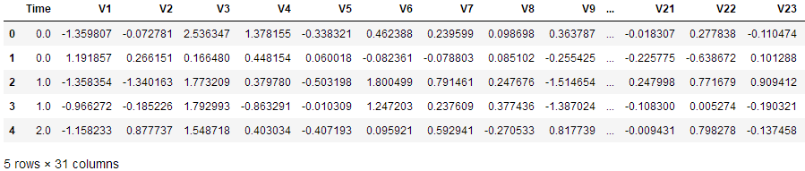
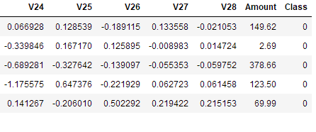
在上图中Class标签代表数据分类，0代表正常数据，1代表欺诈数据。 

这里是做信用卡数据的欺诈检测。在整个数据里面，有正常的数据，也有问题的数据。对于一般情况来说，有问题的数据肯定只占了极少部分。

下面绘出柱状图可以直观显示正常数据与异常数据的数量差异。　　

count_classes = pd.value_counts(data['Class'], sort=True).sort_index()
count_classes.plot(kind='bar') # 使用pandas可以绘制一些简单的图
# 欺诈类别柱状图
plt.title("Fraud class histogram")
plt.xlabel("Class")
# 频率
plt.ylabel("Frequency")

　　

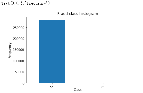
从输出的结果可以看出正常的样本0大概有28万个，异常的样本1非常少，从图中不太容易看出来，但是实际上是存在的，大概只有那么几百个。

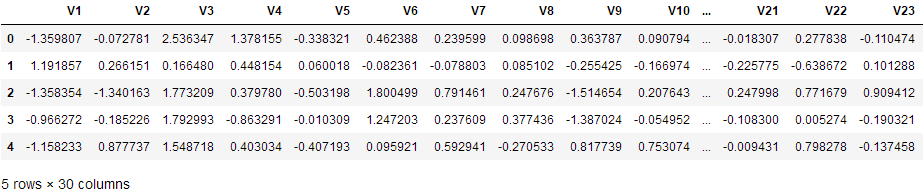
因为Amount这列的数据浮动太大，在做机器学习的过程中，需要保证特征值差异不能过大，于是需要对Amount进行预处理，标准化数据。

Time这一列本身没有多大用处，Amount这一列被标准化后的数据代替。所有删除这两列的数据。

# 预处理  标准化数据
from sklearn.preprocessing import StandardScaler
# norm 标准  -1表示自动判断X维度  对比源码 这里要加上.values
# 加上新的特征列
data['normAmount'] = StandardScaler().fit_transform(data['Amount'].values.reshape(-1, 1))
data = data.drop(['Time', 'Amount'], axis=1)
data.head()

二、样本数据分布不均衡解决方案

上面说到数据集里面正常数据和异常数据数量差异极大，对于这种样本数据不均衡问题，一般有以下两种策略：

（1）下采样策略：之前统计的结果可以看出0的样本有28万个，而1的样本只有几百个。现在将0的数据也变成几百个就可以了。下采样，是使样本的数据同样少
（2）过采样策略：之前统计的结果可以看出0的样本有28万个，而1的样本只有几百个。0比较多1比较少,对1的样本数据进行生成数列，让生成的数据与0的样本数据一样多。

下面首先采用下采样策略

# loc 基于标签索引  iloc 基于行号索引
# ix 基于行号和标签索引都行  但是已被放弃

# X = data.ix[:, data.columns != 'Class']
# # print(X)
# y = data.ix[:, data.columns == 'Class']

X = data.iloc[:, data.columns != 'Class'] # 特征数据
# print(X)
y = data.iloc[:, data.columns == 'Class'] # 

# Number of data points in the minority class 选取少部分异常数据集
number_records_fraud = len(data[data.Class == 1])
fraud_indices = np.array(data[data.Class == 1].index)

# Picking the indices of the normal classes 选取正常类的索引
normal_indices = data[data.Class == 0].index

# Out of the indices we picked, randomly select "x" number (number_records_fraud)
# 从正常类的索引中随机选取 X 个数据  replace 代替的意思
random_normal_indices = np.random.choice(normal_indices,
                                         number_records_fraud,
                                         replace=False)
random_normal_indices = np.array(random_normal_indices)

# Appending the 2 indices
under_sample_indices = np.concatenate([fraud_indices, random_normal_indices])

# Under sample dataset
under_sample_data = data.iloc[under_sample_indices, :]

X_undersample = under_sample_data.iloc[:, under_sample_data.columns != 'Class']
y_undersample = under_sample_data.iloc[:, under_sample_data.columns == 'Class']

# Showing ratio   transactions:交易
print(
    "Percentage of normal transactions:",
    len(under_sample_data[under_sample_data.Class == 0]) /
    len(under_sample_data))
print(
    "Percentage of fraud transactions:",
    len(under_sample_data[under_sample_data.Class == 1]) /
    len(under_sample_data))
print("Total number of transactions in resampled data:",
      len(under_sample_data))

Percentage of normal transactions: 0.5
Percentage of fraud transactions: 0.5
Total number of transactions in resampled data: 984

可以看出经过下采样策略过后，正常数据与异常数据各占50%，并且总样本数也只有少部分。

下面对原始数据集和下采样后的数据集分别进行切分操作。

# sklearn更新后在执行以下代码时可能会出现这样的问题：
# from sklearn.cross_validation import train_test_split
# ModuleNotFoundError: No module named 'sklearn.cross_validation'
# 原因新版本已经不支持 改为以下代码
from sklearn.model_selection import train_test_split

# Whole dataset  test_size 表示训练集测试集的比例  
X_train, X_test, y_train, y_test = train_test_split(X,
                                                    y,
                                                    test_size=0.3,
                                                    random_state=0)

print("Number transactions train dataset:", len(X_train))
print("Number transactions test dataset:", len(X_test))
print("Total number of transactions:", len(X_train) + len(X_test))

# Undersampled dataset
X_train_undersample, X_test_undersample, y_train_undersample, y_test_undersample = train_test_split(
    X_undersample, y_undersample, test_size=0.3, random_state=0)

print("")
print("Number transactions train dataset:", len(X_train_undersample))
print("Number transactions test dataset:", len(X_test_undersample))
print("Total number of transactions:", len(X_train_undersample) + len(X_test_undersample))

Number transactions train dataset: 199364
Number transactions test dataset: 85443
Total number of transactions: 284807

Number transactions train dataset: 688
Number transactions test dataset: 296
Total number of transactions: 984

三、模型评估方法：

假设有1000个病人的数据，有990个人不患癌症，10个人是患癌症。用一个最常见的评估标准，比方说精度，就是真实值与预测值之间的差异，真实值用y来表示，预测值用y1来表示。y真实值1，2，3...10,共有10个样本，y1预测值1，2，3...10，共有10个样本，精度就是看真实值y与预测值y1是否一样的，要么都是0，要么都是1，如果是一致，就用“=”表示，比如1号真实值样本=预测值的1号样本,如果不相等就用不等号来表示。如果等号出现了8个，那么它的精确度为8/10=80%,从而确定模型的精度。

990个人不患癌症，10个人是患癌症建立一个模型，所有的预测值都会建立一个正样本。对1000个样本输入到模型,它的精确度是多少呢?990/1000=99%。这个模型把所有的值都预测成正样本，但是没有得到任何一个负样本。在医院是想得到癌症的识别，但是检查出来的结果是0个，虽然精度达到了99%，但这个模型是没有任何的含义的，因为一个癌症病人都找不出来。在建立模型的时候一定要想好一件事，模型虽然很容易建立出来，那么难点是应该怎么样去评估这样的模型呢?

刚才提到了用精度去评估模型，但是精度有些时候是骗人的。尤其是在样本数据不均衡的情况下。接下来要讲到一个知识点叫recall，叫召回率或叫查全率。recall有0或者1，我们的目标是找出患有癌症的那10个人。因此根据目标制定衡量的标准，就是有10个癌症病人，能够检测出来有几个?如果检测0个癌症病人，那么recall值就是0/10=0。如果检测2个癌症病人，那么recall值就是2/10=20%。用recall检测模型的效果更科学一些。建立模型无非是选择一些参数，recall的表示也并非那么容易.在统计学中会经常提到的4个词，分别如下：

　　

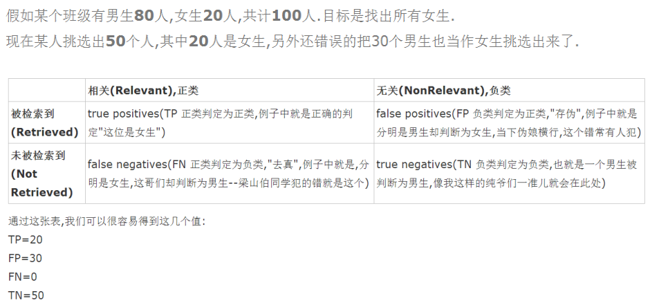
# Recall = TP/(TP+FN) Recall(召回率或查全率)
from sklearn.linear_model import LogisticRegression  # 使用逻辑回归模型
# from sklearn.cross_validation import KFold, cross_val_score  版本更新这行代码也不再支持
from sklearn.model_selection import KFold, cross_val_score  # fold:折叠 KFold 表示切分成几分数据进行交叉验证
from sklearn.metrics import confusion_matrix, recall_score, classification_report

四、正则化惩罚：

比如有A模型的权重参数：θ1、θ2、θ3...θ10，比如还有B模型的权重参数：θ1、θ2、θ3...θ10，这两个模型的recall值都是等于90%。如果两个模型的recall值都是等于90%，是不是随便选一个都可以呢？
但是假如A模型的参数浮动比较大，具体如截图：

　　

B模型的参数浮动较小，如截图所示：

　　

虽然两个模型的recall值都是等于90%，但是A模型的浮动范围太大了，我们希望模型更加稳定一些，不光满足训练的数据，还要尽可能的满足测试数据。因此希望模型的浮动差异更小一些，差异小可以使过度拟合的风险更小一些。

过度拟合的意思是在训练集表达效果很好，但是在测试集表达效果很差，因此这组模型发生了过拟合。过拟合是非常常见的现象，很大程度上是因为权重参数浮动较大引起的，因此希望得到B模型，因为B模型的浮动差异比较小。那么怎么样能够得到B模型呢？从而就引入了正则化的东西，惩罚模型参数θ，因为模型的数据有时候分布大，有时候分布小。希望大力度惩罚A模型，小力度惩罚B模型。我们可以利用正则化找到更为简洁的描述方式的量化过程，我们将损失函数改造为：

　　

C₀表示未引入正则化惩罚之前的损失函数，C表示引入正则化惩罚后新的损失函数，w代表权重参数值。上面这个式子表达的是L1正则化。对于A模型，w值浮动比较大，如果计算|w|的话，这样的话计算的目标损失函数的值就会更大。所有就加上λ参数来惩罚这个权重值。下面还有一种L2正则化。

　　

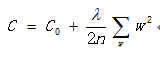
于是最主要就是需要设置当前惩罚的力度到底有多大？可以设置成0.1，那么惩罚力度就比较小，也可以设置惩罚力度为1，也可以设置惩罚力度为10。但是惩罚力度等于多少的时候，效果比较好呢？具体多少也不知道，需要通过交叉验证，去评估一下什么样的参数达到更好的效果。C_param_range = [0.01,0.1,1,10,100]这里就是前面提到的λ参数。需要将这5个参数不断的尝试。

五、交叉验证　　

比如有个集合叫data，通常建立机器模型的时候，先对数据进行切分或者选择，取前面80%的数据当成训练集，取20%的数据当成测试集。80%的数据是来建立一个模型，剩下的20%的数据是用来测试模型。因此第一步是将数据进行切分，切分成训练集以及测试集。这部分操作是必须要做的。第二步还要在训练集进行平均切分，比如平均切分成3份，分别是数据集1,2,3。

在建立模型的时候，不管建立什么样的模型，这个模型伴随着很多参数，有不同的参数进行选择，这个参数选择大比较好，还是选择小比较好一些？从经验值角度来说，肯定没办法很准的，怎么样去确定这个参数呢？只能通过交叉验证的方式。

那什么又叫交叉验证呢？

第一次：将数据集1,2分别建立模型，用数据集3在当前权重下去验证当前模型的效果。数据集3是个验证集，验证集是训练集的一部分。用验证集去验证模型是好还是坏。
第二次：将数据集1,3分别建立模型，用数据集2在当前权重下去验证当前模型的效果。
第三次：将数据集2,3分别建立模型，用数据集1在当前权重下去验证当前模型的效果。

如果只是求一次的交叉验证，这样的操作会存在风险。比如只做第一次交叉验证，会使3验证集偏简单一些。会使模型效果偏高，此外模型有些数据是错误值以及离群值，如果把这些不太好的数据当成验证集，会使模型的效果偏低的。模型当然是不希望偏高也不希望偏低，那就需要多做几次交叉验证模型，求平均值。这里有1，2，3分别作验证集，每个验证集都有评估的标准。最终模型的效果将1，2，3的评估效果加在一起，再除以3，就可以得到模型一个大致的效果。

def printing_Kfold_scores(x_train_data,y_train_data):
    fold = KFold(5,shuffle=False)
    
    # Different C parameters
    c_param_range = [0.01,0.1,1,10,100]
    
    result_table = pd.DataFrame(index=range(len(c_param_range),2),columns=['C_parameter','Mean recall score'])
    result_table['C_parameter'] = c_param_range
    
    # the k-fold will give 2 lists:train_indices=indices[0],test_indices = indices[1]
    j=0  # 循环找到最好的惩罚力度
    for c_param in c_param_range:
        print('-------------------------------------------')
        print('C parameter:',c_param)
        print('-------------------------------------------')
        print('')
        
        recall_accs = []
        for iteration,indices in enumerate(fold.split(x_train_data)):
            
            # 使用特定的C参数调用逻辑回归模型
            # Call the logistic regression model with a certain C parameter
            # 参数 solver=’liblinear’ 消除警告
            # 出现警告：模型未能收敛 ，请增加收敛次数
            #  ConvergenceWarning: Liblinear failed to converge, increase the number of iterations.
            #  "the number of iterations.", ConvergenceWarning)
            #  增加参数 max_iter 默认1000
            lr = LogisticRegression(C = c_param, penalty='l1', solver='liblinear',max_iter=10000)
            # Use the training data to fit the model. In this case, we use the portion
            # of the fold to train the model with indices[0], We then predict on the
            # portion assigned as the 'test cross validation' with indices[1]
            lr.fit(x_train_data.iloc[indices[0],:],y_train_data.iloc[indices[0],:].values.ravel())
            
            # Predict values using the test indices in the training data
            y_pred_undersample = lr.predict(x_train_data.iloc[indices[1],:].values)
            
            # Calculate the recall score and append it to a list for recall scores 
            # representing the current c_parameter
            recall_acc = recall_score(y_train_data.iloc[indices[1],:].values,y_pred_undersample)
            recall_accs.append(recall_acc)
            print('Iteration ',iteration,': recall score = ',recall_acc)
            
        # the mean value of those recall scores is the metric we want to save and get
        # hold of.
        result_table.loc[j,'Mean recall score'] = np.mean(recall_accs)
        j += 1
        print('')
        print('Mean recall score ',np.mean(recall_accs))
        print('')
        
    # 注意此处报错  源代码没有astype('float64')
    best_c = result_table.loc[result_table['Mean recall score'].astype('float64').idxmax()]['C_parameter']
    # Finally, we can check which C parameter is the best amongst the chosen.
    print('*********************************************************************************')
    print('Best model to choose from cross validation is with C parameter',best_c)
    print('*********************************************************************************')
    
    return best_c

使用下采样数据集调用上面这个函数　　

best_c = printing_Kfold_scores(X_train_undersample,y_train_undersample)

 输出结果：

-------------------------------------------
C parameter: 0.01
-------------------------------------------

Iteration  0 : recall score =  0.958904109589041
Iteration  1 : recall score =  0.9178082191780822
Iteration  2 : recall score =  1.0
Iteration  3 : recall score =  0.9864864864864865
Iteration  4 : recall score =  0.9545454545454546

Mean recall score  0.9635488539598128

-------------------------------------------
C parameter: 0.1
-------------------------------------------

Iteration  0 : recall score =  0.8356164383561644
Iteration  1 : recall score =  0.863013698630137
Iteration  2 : recall score =  0.9322033898305084
Iteration  3 : recall score =  0.9459459459459459
Iteration  4 : recall score =  0.8939393939393939

Mean recall score  0.8941437733404299

-------------------------------------------
C parameter: 1
-------------------------------------------

Iteration  0 : recall score =  0.8493150684931506
Iteration  1 : recall score =  0.863013698630137
Iteration  2 : recall score =  0.9830508474576272
Iteration  3 : recall score =  0.9459459459459459
Iteration  4 : recall score =  0.9090909090909091

Mean recall score  0.9100832939235539

-------------------------------------------
C parameter: 10
-------------------------------------------

Iteration  0 : recall score =  0.863013698630137
Iteration  1 : recall score =  0.863013698630137
Iteration  2 : recall score =  0.9830508474576272
Iteration  3 : recall score =  0.9324324324324325
Iteration  4 : recall score =  0.9242424242424242

Mean recall score  0.9131506202785514

-------------------------------------------
C parameter: 100
-------------------------------------------

Iteration  0 : recall score =  0.863013698630137
Iteration  1 : recall score =  0.863013698630137
Iteration  2 : recall score =  0.9830508474576272
Iteration  3 : recall score =  0.9459459459459459
Iteration  4 : recall score =  0.9242424242424242

Mean recall score  0.9158533229812542

*********************************************************************************
Best model to choose from cross validation is with C parameter 0.01
*********************************************************************************

根据上面结果可以看出，当正则化参数为0.01时，recall的值最高。

未完待续。。。