翻译自《Demo Week: Tidy Forecasting with sweep》
原文链接:www.business-science.io/code-tools/2017/10/25/demo_week_sweep.html
时间序列分析工具箱——sweep

sweep 的用途
正如 broom 包之于 stats 包,sweep 包用来简化使用 forecast 包的工作流。本教程将逐一介绍常用函数 sw_tidy、sw_glance、sw_augment 和 sw_sweep 的用法。
sweep 和 timetk 带来的额外好处是,如果 ts 对象是由 tbl 对象转换来的,那么在预测过程中日期和时间信息会以 timetk 索引的形式保留下来。一句话概括:这意味着我们最终可以在预测时使用日期,而不是 ts 类型数据使用的规则间隔数字日期。
加载包
本教程要使用到四个包:
sweep:简化forecast包的使用forecast:提供 ARIMA、ETS 和其他流行的预测算法tidyquant:获取数据并在后台加载tidyverse系列工具timetk:时间序列数据处理工具,用来将tbl转换成ts
# Load libraries
library(sweep)      # Broom-style tidiers for the forecast package
library(forecast)   # Forecasting models and predictions package
library(tidyquant)  # Loads tidyverse, financial pkgs, used to get data
library(timetk)     # Functions working with time series
数据
我们使用 timetk 教程中数据——啤酒、红酒和蒸馏酒销售数据,用 tidyquant 中的 tq_get() 函数从 FRED 获取。
# Beer, Wine, Distilled Alcoholic Beverages, in Millions USD
beer_sales_tbl <- tq_get(
    "S4248SM144NCEN",
    get = "economic.data",
    from = "2010-01-01",
    to = "2016-12-31")

beer_sales_tbl
## # A tibble: 84 x 2
##          date price
##        <date> <int>
##  1 2010-01-01  6558
##  2 2010-02-01  7481
##  3 2010-03-01  9475
##  4 2010-04-01  9424
##  5 2010-05-01  9351
##  6 2010-06-01 10552
##  7 2010-07-01  9077
##  8 2010-08-01  9273
##  9 2010-09-01  9420
## 10 2010-10-01  9413
## # ... with 74 more rows
可视化数据是一个好东西,这有助于帮助我们了解正在使用的是什么数据。可视化对于时间序列分析和预测尤为重要。我们将使用 tidyquant 画图工具:主要是用 geom_ma(ma_fun = SMA,n = 12) 来添加一个周期为 12 的简单移动平均线来了解趋势。我们还可以看到似乎同时存在着趋势性(移动平均线以近似线性的模式增长)和季节性(波峰和波谷倾向于在特定月份发生)。
# Plot Beer Sales
beer_sales_tbl %>%
    ggplot(aes(date, price)) +
    geom_line(col = palette_light()[1]) +
    geom_point(col = palette_light()[1]) +
    geom_ma(ma_fun = SMA, n = 12, size = 1) +
    theme_tq() +
    scale_x_date(date_breaks = "1 year", date_labels = "%Y") +
    labs(title = "Beer Sales: 2007 through 2016")
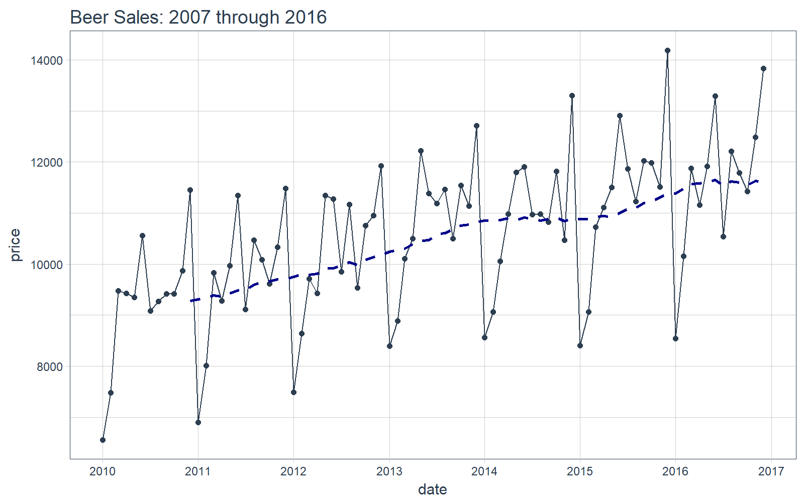
现在你对我们要分析的时间序列有了直观的感受,那么让我们继续!
Demo:forecast + sweep 的简化预测工作流
我们将联合使用 forecast 和 sweep 来简化预测分析。
关键想法:使用 forecast 包做预测涉及到 ts 对象,用起来并不简洁。对于 stats 包来说有 broom 来简化使用;forecast 包就用 sweep。
目标:我们将用 ARIMA 模型预测未来 12 个月的数据。
STEP 1:创建 ts 对象
使用 timetk::tk_ts() 将 tbl 转换成 ts,从之前的教程可以了解到这个函数有两点好处:
- 这是一个统一的方法,实现与
ts对象的相互转换。 - 得到的
ts对象包含timetk_idx属性,是一个基于初始时间信息的索引。
下面开始转换,注意 ts 对象是规则时间序列,所以要设置 start 和 freq。
# Convert from tbl to ts
beer_sales_ts <- tk_ts(
    beer_sales_tbl,
    start = 2010,
    freq = 12)

beer_sales_ts
##        Jan   Feb   Mar   Apr   May   Jun   Jul   Aug   Sep   Oct
## 2010  6558  7481  9475  9424  9351 10552  9077  9273  9420  9413
## 2011  6901  8014  9833  9281  9967 11344  9106 10468 10085  9612
## 2012  7486  8641  9709  9423 11342 11274  9845 11163  9532 10754
## 2013  8395  8888 10109 10493 12217 11385 11186 11462 10494 11541
## 2014  8559  9061 10058 10979 11794 11906 10966 10981 10827 11815
## 2015  8398  9061 10720 11105 11505 12903 11866 11223 12023 11986
## 2016  8540 10158 11879 11155 11916 13291 10540 12212 11786 11424
##        Nov   Dec
## 2010  9866 11455
## 2011 10328 11483
## 2012 10953 11922
## 2013 11139 12709
## 2014 10466 13303
## 2015 11510 14190
## 2016 12482 13832
检查 ts 对象具有 timetk_idx 属性。
# Check that ts-object has a timetk index
has_timetk_idx(beer_sales_ts)
## [1] TRUE
OK,这对后面要用的 sw_sweep() 很重要。下面我们就要建立 ARIMA 模型了。
STEP 2A:ARIMA 模型
我们使用 forecast 包里的 auto.arima() 函数为时间序列建模。
# Model using auto.arima
fit_arima <- auto.arima(beer_sales_ts)

fit_arima
## Series: beer_sales_ts
## ARIMA(3,0,0)(1,1,0)[12] with drift
##
## Coefficients:
##           ar1     ar2     ar3     sar1    drift
##       -0.2498  0.1079  0.6210  -0.2817  32.1157
## s.e.   0.0933  0.0982  0.0925   0.1333   5.8882
##
## sigma^2 estimated as 175282:  log likelihood=-535.49
## AIC=1082.97   AICc=1084.27   BIC=1096.63
STEP 2B:简化模型
就像 broom 简化 stats 包的使用一样,我么可以使用 sweep 的函数简化 ARIMA 模型。下面介绍三个函数:
sw_tidy():用于检索模型参数sw_glance():用于检索模型描述和训练集的精确度度量sw_augment():用于获得模型残差
sw_tidy
sw_tidy() 函数以 tibble 对象的形式返回模型参数。
# sw_tidy - Get model coefficients
sw_tidy(fit_arima)
## # A tibble: 5 x 2
##    term   estimate
##   <chr>      <dbl>
## 1   ar1 -0.2497937
## 2   ar2  0.1079269
## 3   ar3  0.6210345
## 4  sar1 -0.2816877
## 5 drift 32.1157478
sw_glance
sw_glance() 函数以 tibble 对象的形式返回训练集的精确度度量。可以使用 glimpse 函数美化显示结果。
# sw_glance - Get model description and training set accuracy measures
sw_glance(fit_arima) %>%
    glimpse()
## Observations: 1
## Variables: 12
## $ model.desc <chr> "ARIMA(3,0,0)(1,1,0)[12] with drift"
## $ sigma      <dbl> 418.6665
## $ logLik     <dbl> -535.4873
## $ AIC        <dbl> 1082.975
## $ BIC        <dbl> 1096.635
## $ ME         <dbl> 1.189875
## $ RMSE       <dbl> 373.9091
## $ MAE        <dbl> 271.7068
## $ MPE        <dbl> -0.06716239
## $ MAPE       <dbl> 2.526077
## $ MASE       <dbl> 0.4989005
## $ ACF1       <dbl> 0.02215405
sw_augument
sw_augument() 函数返回的 tibble 表中包含 .actual、.fitted 和 .resid 列,有助于在训练集上评估模型表现。注意,设置 timetk_idx = TRUE 返回初始的日期索引。
# sw_augment - get model residuals
sw_augment(fit_arima, timetk_idx = TRUE)
## # A tibble: 84 x 4
##         index .actual   .fitted    .resid
##        <date>   <dbl>     <dbl>     <dbl>
##  1 2010-01-01    6558  6551.474  6.525878
##  2 2010-02-01    7481  7473.583  7.416765
##  3 2010-03-01    9475  9465.621  9.378648
##  4 2010-04-01    9424  9414.704  9.295526
##  5 2010-05-01    9351  9341.810  9.190414
##  6 2010-06-01   10552 10541.641 10.359293
##  7 2010-07-01    9077  9068.148  8.852178
##  8 2010-08-01    9273  9263.984  9.016063
##  9 2010-09-01    9420  9410.869  9.130943
## 10 2010-10-01    9413  9403.908  9.091831
## # ... with 74 more rows
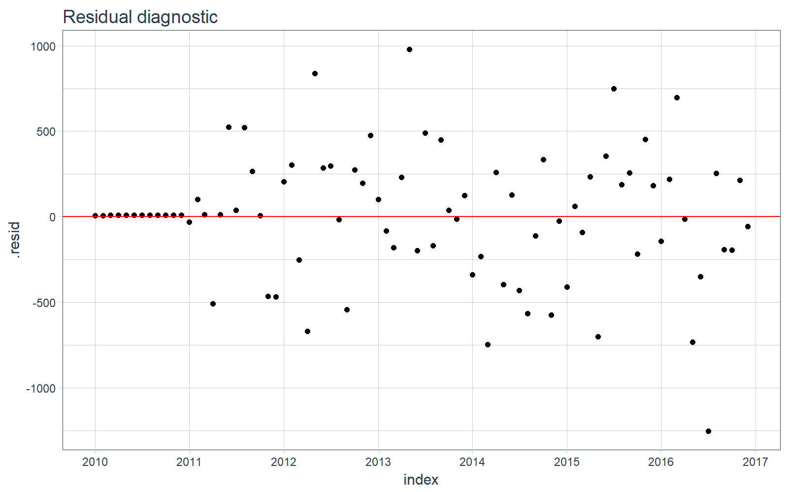
我们可以可视化训练数据上的残差,看一下数据中有没有遗漏的模式没有被发现。
# Plotting residuals
sw_augment(fit_arima, timetk_idx = TRUE) %>%
    ggplot(aes(x = index, y = .resid)) +
    geom_point() +
    geom_hline(yintercept = 0, color = "red") +
    labs(title = "Residual diagnostic") +
    scale_x_date(date_breaks = "1 year", date_labels = "%Y") +
    theme_tq()
STEP 3:预测
使用 forecast() 函数做预测。
# Forecast next 12 months
fcast_arima <- forecast(fit_arima, h = 12)
一个问题是,预测结果并不“tidy”。我们需要数据框形式的预测结果,以便应用 tidyverse 的功能,然而预测结果是 forecast 类型的,一种基于 ts 的对象。
class(fcast_arima)
## [1] "forecast"
STEP 4:用 sweep 简化预测
我们使用 sw_sweep() 简化预测结果,一个额外的好处是,如果 forecast 对象有 timetk 索引,我们可以用它返回一个日期时间索引,不同于 ts 对象的规则索引。
首先要确认 forecast 对象有 timetk 索引,这需要在使用 sw_sweep() 时设置 timetk_idx 参数。
# Check if object has timetk index
has_timetk_idx(fcast_arima)
## [1] TRUE
现在,使用 sw_sweep() 来简化预测结果,它会在内部根据 time_tk 构造一条未来时间序列索引(这一步总是会被执行,因为我们在第 1 步中用 tk_ts() 构造了 ts 对象)注意:这意味着我们最终可以在 forecast 包中使用日期(不同于 ts 对象中的规则索引)!。
# sw_sweep - tidies forecast output
fcast_tbl <- sw_sweep(fcast_arima, timetk_idx = TRUE)

fcast_tbl
## # A tibble: 96 x 7
##         index    key price lo.80 lo.95 hi.80 hi.95
##        <date>  <chr> <dbl> <dbl> <dbl> <dbl> <dbl>
##  1 2010-01-01 actual  6558    NA    NA    NA    NA
##  2 2010-02-01 actual  7481    NA    NA    NA    NA
##  3 2010-03-01 actual  9475    NA    NA    NA    NA
##  4 2010-04-01 actual  9424    NA    NA    NA    NA
##  5 2010-05-01 actual  9351    NA    NA    NA    NA
##  6 2010-06-01 actual 10552    NA    NA    NA    NA
##  7 2010-07-01 actual  9077    NA    NA    NA    NA
##  8 2010-08-01 actual  9273    NA    NA    NA    NA
##  9 2010-09-01 actual  9420    NA    NA    NA    NA
## 10 2010-10-01 actual  9413    NA    NA    NA    NA
## # ... with 86 more rows
STEP 5:比较真实值和预测值
我们可以使用 tq_get() 来检索实际数据。注意,我们没有用于比较的完整数据,但我们至少可以比较前几个月的实际值。
actuals_tbl <- tq_get(
    "S4248SM144NCEN",
    get = "economic.data",
    from = "2017-01-01",
    to = "2017-12-31")
注意,预测结果放在 tibble 中,可以方便的实现可视化。
# Visualize the forecast with ggplot
fcast_tbl %>%
    ggplot(
        aes(x = index, y = price, color = key)) +
    # 95% CI
    geom_ribbon(
        aes(ymin = lo.95, ymax = hi.95),
        fill = "#D5DBFF", color = NA, size = 0) +
    # 80% CI
    geom_ribbon(
        aes(ymin = lo.80, ymax = hi.80, fill = key),
        fill = "#596DD5", color = NA,
        size = 0, alpha = 0.8) +
    # Prediction
    geom_line() +
    geom_point() +
    # Actuals
    geom_line(
        aes(x = date, y = price), color = palette_light()[[1]],
        data = actuals_tbl) +
    geom_point(
        aes(x = date, y = price), color = palette_light()[[1]],
        data = actuals_tbl) +
    # Aesthetics
    labs(
        title = "Beer Sales Forecast: ARIMA", x = "", y = "Thousands of Tons",
        subtitle = "sw_sweep tidies the auto.arima() forecast output") +
    scale_x_date(
        date_breaks = "1 year",
        date_labels = "%Y") +
    scale_color_tq() +
    scale_fill_tq() +
    theme_tq()
我们可以研究测试集上的误差(真实值 vs 预测值)。
# Investigate test error
error_tbl <- left_join(
    actuals_tbl,
    fcast_tbl,
    by = c("date" = "index")) %>%
    rename(
        actual = price.x, pred = price.y) %>%
    select(date, actual, pred) %>%
    mutate(
        error     = actual - pred,
        error_pct = error / actual)

error_tbl
## # A tibble: 8 x 5
##         date actual      pred      error    error_pct
##       <date>  <int>     <dbl>      <dbl>        <dbl>
## 1 2017-01-01   8664  8601.815   62.18469  0.007177365
## 2 2017-02-01  10017 10855.429 -838.42908 -0.083700617
## 3 2017-03-01  11960 11502.214  457.78622  0.038276439
## 4 2017-04-01  11019 11582.600 -563.59962 -0.051147982
## 5 2017-05-01  12971 12566.765  404.23491  0.031164514
## 6 2017-06-01  14113 13263.918  849.08191  0.060163106
## 7 2017-07-01  10928 11507.277 -579.27693 -0.053008504
## 8 2017-08-01  12788 12527.278  260.72219  0.020388035
并且,我们可以做简单的误差度量。MAPE 接近 4.3%,比简单的线性回归模型略好一点,但是 RMSE 变差了。
# Calculate test error metrics
test_residuals <- error_tbl$error
test_error_pct <- error_tbl$error_pct * 100 # Percentage error

me   <- mean(test_residuals, na.rm=TRUE)
rmse <- mean(test_residuals^2, na.rm=TRUE)^0.5
mae  <- mean(abs(test_residuals), na.rm=TRUE)
mape <- mean(abs(test_error_pct), na.rm=TRUE)
mpe  <- mean(test_error_pct, na.rm=TRUE)

tibble(me, rmse, mae, mape, mpe) %>%
    glimpse()
## Observations: 1
## Variables: 5
## $ me   <dbl> 6.588034
## $ rmse <dbl> 561.4631
## $ mae  <dbl> 501.9144
## $ mape <dbl> 4.312832
## $ mpe  <dbl> -0.3835956