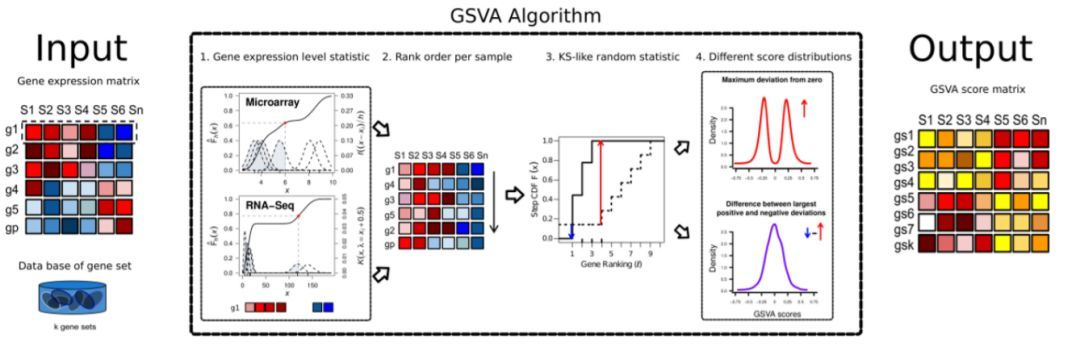
大家应该对通路富集分析都很熟悉,如DAVID、超几何富集分析等。都是在大量文章中常见的通路富集方法,给大家介绍一个更加复杂的通路富集分析的前期数据处理包GSVA(gene set variation analysis)与gsea选择。GSVA是一种非参数的无监督分析方法,主要用来评估芯片核转录组的基因集富集结果。主要是通过将基因在不同样品间的表达量矩阵转化成基因集在样品间的表达量矩阵,从而来评估不同的通路在不同样品间是否富集。具体的一个分析流程如下:
1. 超几何检验GO、KEGG基因富集分析
这是相对简单粗暴一些的基因富集分析方法,不需要输入基因的表达值,只需要通过自己设定的阈值(|log2FC| >1 和Pvalue < 0.05)筛选得到的差异基因名。进行统计检验后返回显著富集的功能基因集。如DESeq2 (获得差异基因信息),clusterProfiler(ID转换+富集分析+作图一站式神包!)
2. GSEA富集分析
相比于第一种简单粗暴的用硬阈值截取+往篮子里塞鸡蛋的方法,GSEA同时考虑了基因在整个表达谱中所处的FoldChange rank以及同一基因集中的基因在表达谱rank中的距离。通俗来讲,GSEA基于如下假设:一个基因集中的基因如果在表达谱中所处的rank越极端(高/低FoldChange),而且基因之间的距离越短(rank相近),则这个基因集越可能显著。所以GSEA需要输入的是【所有纳入差异分析的完整基因list和它们的FC值,并已经预先排序(pre-ranked)】。
具体的原理参考,https://cloud.tencent.com/developer/article/1426130
3. GSVA/ssGSEA分析
ssGSEA顾名思义是一种特殊的GSEA,它主要针对单样本无法做GSEA而提出的一种实现方法,原理上与GSEA是类似的,不同的是GSEA需要准备表达谱文件即gct,根据表达谱文件计算每个基因的rank值,再进行后续的统计分析。ssGSEA是为无重复的样本进行,geneset enrichment analysis准备的,所以不同于上方以组别为单位(cancer vs normal)的GSEA分析,通过ssGSEA,每个样本都可以得到相应基因集的评分。
a. 首先假设有一个样本的表达数据,那么他应该是这样的,第一列为基因,第二列为表达值,这样的两列的数据矩阵。
首先对样本的所有基因的表达水平进行排序获得其在所有基因中的秩次rank,这些基因的集合为BG。
b. 假设要对其进行KEGG的分析,首先我们需要在GSEA官网找到KEGG对应的gmt文件。
gmt文件主要格式是:每行表示一个通路,第一列为通路ID,第二列为通路对应的描述,第三列开始到最后一列为该通路中的基因。
c. 那么对于任意的一个通路A,我们可以拿到这个通路的基因列表GL,从GL中寻找BG里存在的基因并计数为NC,并将这些基因的表达水平加和为SG。
开始计算ES:对于任意一个表达谱中的基因 G,如果G是集合GL中的基因则他的ES等于该基因的表达水平除以SG,否则记该基因的ES等于1除以(基因集合BG总个数减去NC)
依次计算每个BG中的基因的ES值,找到其中绝对值最大的ES作为通路A的A.ES
d. 到此通路A的ES计算完毕,需要一个统计学方法来评估该ES是否是显著的,即非随机的。
按照上述计算ES的方法,先随机打乱表达谱中基因的表达顺序,然后再依次计算ES值,如此重复一千次,得到一千个ES值,我们根据这一千个ES值的分布,来计算A.ES在这个分布中所处的位置及出现在该位置时的概率即得到了p值 。依次分别计算每个通路的ES及p值,然后使用多重检验矫正得到每个通路的FDR
此外,对于多个样本或多组样本,也可以利用T检验或方差检验对结果进行p值的计算与相应的FDR值。
以上即是整个ssGSEA算法的整体思路。
R语言,GSVA包(进行GSVA/ssGSEA分析),limma包(差异pathway的筛选),pheatmap包(热图绘制)。
library(GSEABase)
library(GSVA)
#读取基因集文件
geneSets <- getGmt("test.geneset")
#读取表达量文件并去除重复
mydata <- read.table(file = "all.genes.fpkm.xls",header=T)
name=mydata[,1]
index <- duplicated(mydata[,1])
fildup=mydata[!index,]
exp=fildup[,-1]
row.names(exp)=name
#将数据框转换成矩阵
mydata= as.matrix(exp)
#使用gsva方法进行分析,默认mx.diff=TRUE,min.sz=1,max.zs=Inf,这里是设置最小值和最大值
res_es <- gsva(mydata, geneSets, min.sz=10, max.sz=500, verbose=FALSE, parallel.sz=1)
pheatmap(res_es)
Usage
## S4 method for signature 'ExpressionSet,list'
gsva(expr, gset.idx.list, annotation,method=c("gsva", "ssgsea", "zscore", "plage"),
kcdf=c("Gaussian", "Poisson", "none"),abs.ranking=FALSE,min.sz=1,max.sz=Inf,
parallel.sz=0,parallel.type="SOCK",mx.diff=TRUE,tau=switch(method, gsva=1, ssgsea=0.25, NA),ssgsea.norm=TRUE,verbose=TRUE)
Arguments
expr
Gene expression data which can be given either as an ExpressionSet object or as a matrix of expression values where rows correspond to genes and columns correspond to samples.
gset.idx.list
Gene sets provided either as a list object or as a GeneSetCollection object.
annotation
In the case of calling gsva() with expression data in a matrix and gene sets as a GeneSetCollection object, the annotation argument can be used to supply the name of the Bioconductor package that contains annotations for the class of gene identifiers occurring in the row names of the expression data matrix. By default gsva() will try to match the identifiers in expr to the identifiers in gset.idx.list just as they are, unless the annotation argument is set.
method
Method to employ in the estimation of gene-set enrichment scores per sample. By default this is set to gsva (Hänzelmann et al, 2013) and other options are ssgsea (Barbie et al, 2009), zscore (Lee et al, 2008) or plage (Tomfohr et al, 2005). The latter two standardize first expression profiles into z-scores over the samples and, in the case of zscore, it combines them together as their sum divided by the square-root of the size of the gene set, while in the case of plage they are used to calculate the singular value decomposition (SVD) over the genes in the gene set and use the coefficients of the first right-singular vector as pathway activity profile.
kcdf
Character string denoting the kernel to use during the non-parametric estimation of the cumulative distribution function of expression levels across samples when method="gsva". By default, kcdf="Gaussian" which is suitable when input expression values are continuous, such as microarray fluorescent units in logarithmic scale, RNA-seq log-CPMs, log-RPKMs or log-TPMs. When input expression values are integer counts, such as those derived from RNA-seq experiments, then this argument should be set to kcdf="Poisson".
abs.ranking
Flag used only when mx.diff=TRUE. When abs.ranking=FALSE (default) a modified Kuiper statistic is used to calculate enrichment scores, taking the magnitude difference between the largest positive and negative random walk deviations. When abs.ranking=TRUE the original Kuiper statistic that sums the largest positive and negative random walk deviations, is used. In this latter case, gene sets with genes enriched on either extreme (high or low) will be regarded as 'highly' activated.
min.sz
Minimum size of the resulting gene sets.
max.sz
Maximum size of the resulting gene sets.
parallel.sz
Number of processors to use when doing the calculations in parallel. This requires to previously load either the parallel or the snow library. If parallel is loaded and this argument is left with its default value (parallel.sz=0) then it will use all available core processors unless we set this argument with a smaller number. If snow is loaded then we must set this argument to a positive integer number that specifies the number of processors to employ in the parallel calculation.
parallel.type
Type of cluster architecture when using snow.
mx.diff
Offers two approaches to calculate the enrichment statistic (ES) from the KS random walk statistic. mx.diff=FALSE: ES is calculated as the maximum distance of the random walk from 0. mx.diff=TRUE (default): ES is calculated as the magnitude difference between the largest positive and negative random walk deviations.
tau
Exponent defining the weight of the tail in the random walk performed by both the gsva (Hänzelmann et al., 2013) and the ssgsea (Barbie et al., 2009) methods. By default, this tau=1 when method="gsva" and tau=0.25 when method="ssgsea" just as specified by Barbie et al. (2009) where this parameter is called alpha.
ssgsea.norm
Logical, set to TRUE (default) with method="ssgsea" runs the SSGSEA method from Barbie et al. (2009) normalizing the scores by the absolute difference between the minimum and the maximum, as described in their paper. When ssgsea.norm=FALSE this last normalization step is skipped.
verbose
Gives information about each calculation step. Default: FALSE.