6.3 Evaluation 评分
In order to decide whether a classification model is accurately capturing a pattern, we must evaluate that model. The result of this evaluation is important for deciding how trustworthy the model is, and for what purposes we can use it. Evaluation can also be an effective tool for guiding us in making future improvements to the model.
The Test Set 测试集
Most evaluation techniques calculate a score for a model by comparing the labels that it generates for the inputs in a test set (or evaluation set) with the correct labels for those inputs. This test set typically has the same format as the training set. However, it is very important that the test set be distinct from the training corpus: if we simply re-used the training set as the test set, then a model that simply memorized its input, without learning how to generalize to new examples, would receive misleadingly(误导的) high scores.
When building the test set, there is often a trade-off between the amount of data available for testing and the amount available for training. For classification tasks that have a small number of well-balanced labels and a diverse test set, a meaningful evaluation can be performed with as few as 100 evaluation instances. But if a classification task has a large number of labels, or includes very infrequent labels, then the size of the test set should be chosen to ensure that the least frequent label occurs at least 50 times. Additionally, if the test set contains many closely related instances — such as instances drawn from(来自) a single document — then the size of the test set should be increased to ensure that this lack of diversity does not skew(歪曲) the evaluation results. When large amounts of annotated data are available, it is common to err on the side of safety by using 10% of the overall data for evaluation.
Another consideration when choosing the test set is the degree of similarity(相似度) between instances in the test set and those in the development set. The more similar these two datasets are, the less confident we can be that evaluation results will generalize to other datasets. For example, consider the part-of-speech tagging task. At one extreme, we could create the training set and test set by randomly assigning sentences from a data source that reflects a single genre (news):
|
In this case, our test set will be very similar to our training set. The training set and test set are taken from the same genre, and so we cannot be confident that evaluation results would generalize to other genres. What's worse, because of the call to random.shuffle(), the test set contains sentences that are taken from the same documents that were used for training. If there is any consistent pattern within a document — say, if a given word appears with a particular part-of-speech tag especially frequently(特别地频繁) — then that difference will be reflected in both the development set and the test set. A somewhat(稍微) better approach is to ensure that the training set and test set are taken from different documents:
|
If we want to perform a more stringent(令人信服的) evaluation, we can draw the test set from documents that are less closely related to those in the training set:
|
If we build a classifier that performs well on this test set, then we can be confident that it has the power to generalize well beyond the data that it was trained on.
Accuracy 精确度
The simplest metric(度量) that can be used to evaluate a classifier, accuracy, measures the percentage of inputs in the test set that the classifier correctly labeled. For example, a name gender classifier that predicts the correct name 60 times in an test set containing 80 names would have an accuracy of 60/80 = 75%. The function nltk.classify.accuracy() will calculate the accuracy of a classifier model on a given test set:
|
When interpreting the accuracy score of a classifier, it is important to take into consideration the frequencies of the individual class labels in the test set. For example, consider a classifier that determines the correct word sense for each occurrence of the word bank. If we evaluate this classifier on financial newswire text, then we may find that the financial-institution sense appears 19 times out of 20. In that case, an accuracy of 95% would hardly be impressive, since we could achieve that accuracy with a model that always returns the financial-institution sense. However, if we instead evaluate the classifier on a more balanced corpus, where the most frequent word sense has a frequency of 40%, then a 95% accuracy score would be a much more positive result. (A similar issue arises when measuring inter-annotator agreement in Section 11.2.)
Precision and Recall 准确率和召回率
Another instance where accuracy scores can be misleading(使人误解的) is in "search" tasks, such as information retrieval, where we are attempting to find documents that are relevant to a particular task. Since the number of irrelevant documents far outweighs(远远超过) the number of relevant documents, the accuracy score for a model that labels every document as irrelevant would be very close to 100%.
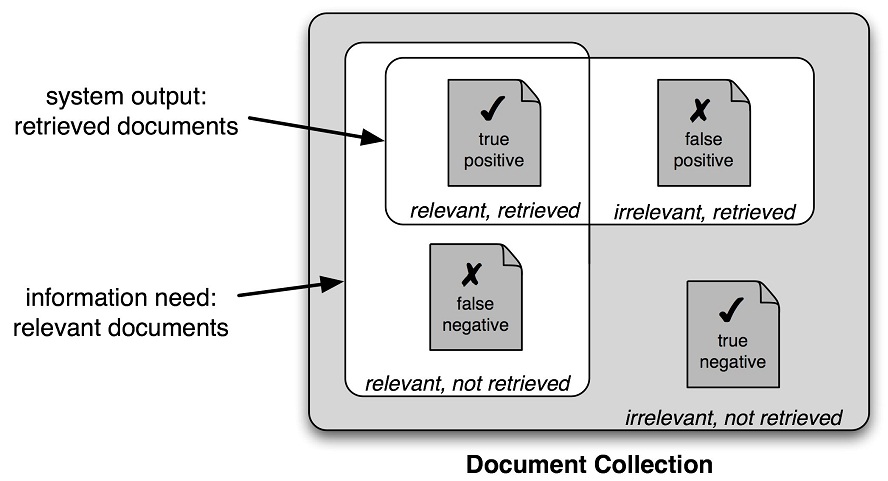
Figure 6.10: True and False Positives and Negatives(很重要的概念)
It is therefore conventional to employ a different set of measures for search tasks, based on the number of items in each of the four categories shown in Figure 6.10:
- True positives are relevant items that we correctly identified as relevant.
- True negatives are irrelevant items that we correctly identified as irrelevant.
- False positives (or Type I errors) are irrelevant items that we incorrectly identified as relevant.
- False negatives (or Type II errors) are relevant items that we incorrectly identified as irrelevant.
Given these four numbers, we can define the following metrics:
- Precision, which indicates how many of the items that we identified were relevant, is TP/(TP+FP).
- Recall, which indicates how many of the relevant items that we identified, is TP/(TP+FN).
- The F-Measure (or F-Score), which combines the precision and recall to give a single score, is defined to be the harmonic mean of the precision and recall: (2 × Precision × Recall) / (Precision + Recall).
Confusion Matrices 混淆矩阵
When performing classification tasks with three or more labels, it can be informative to subdivide(细分) the errors made by the model based on which types of mistake it made. A confusion matrix is a table where each cell [i,j] indicates how often label j was predicted when the correct label was i. Thus, the diagonal(对角线) entries (i.e., cells [i,j]) indicate labels that were correctly predicted, and the off-diagonal(非对角线的) entries indicate errors. In the following example, we generate a confusion matrix for the unigram tagger developed in Section 5.4:
|
The confusion matrix indicates that common errors include a substitution of NN for JJ (for 1.6% of words), and of NN for NNS (for 1.5% of words). Note that periods (.) indicate cells whose value is 0, and that the diagonal entries — which correspond to correct classifications — are marked with angle brackets(尖括号).
Cross-Validation 交叉验证
In order to evaluate our models, we must reserve a portion of(一部分) the annotated data for the test set. As we already mentioned, if the test set is too small, then our evaluation may not be accurate. However, making the test set larger usually means making the training set smaller, which can have a significant impact on performance if a limited amount of annotated data is available.
One solution to this problem is to perform multiple evaluations on different test sets, then to combine the scores from those evaluations, a technique known as cross-validation. In particular, we subdivide the original corpus into N subsets called folds(褶皱?). For each of these folds, we train a model using all of the data except the data in that fold, and then test that model on the fold. Even though the individual folds might be too small to give accurate evaluation scores on their own, the combined evaluation score is based on a large amount of data, and is therefore quite reliable.
A second, and equally important, advantage of using cross-validation is that it allows us to examine how widely the performance varies across different training sets(检查在不同的训练集之间的性能变化有多大). If we get very similar scores for all N training sets, then we can be fairly confident that the score is accurate. On the other hand, if scores vary widely across the N training sets, then we should probably be skeptical(怀疑的) about the accuracy of the evaluation score.