简介
网格简化是图形学中的一项重要操作,可以加深对于图形学的理解
论文
Surface Simplification Using Quadric Error Metrics
实现步骤
算法思路:
- 计算每一个点的 Kp 矩阵
[K_{p}=left(egin{array}{llll}
a^{2} & a b & a c & a d \
a b & b^{2} & b c & b d \
a c & b c & c^{2} & c d \
a d & b d & c d & d^{2}
end{array}
ight)]
2建立最小堆 使用 multiset 建立
3.迭代
a.移动顶点
b.删除顶点
c.增加面
TIPS
1.
[egin{aligned}
Delta(mathbf{v}) &=sum_{mathbf{p} in operatorname{planes}(mathbf{v})}left(mathbf{v}^{ op} mathbf{p}
ight)left(mathbf{p}^{ op} mathbf{v}
ight) \
&=sum_{mathbf{p} in ext { planes }(mathbf{v})} mathbf{v}^{ op}left(mathbf{p} mathbf{p}^{ op}
ight) mathbf{v} \
&=mathbf{v}^{ op}left(sum_{mathbf{p} in ext { planes }(mathbf{v})} mathbf{K}_{mathbf{p}}
ight) mathbf{v}
end{aligned}]
上式 其实就是 Q 二次误差的计算方式
2.
[overline{mathbf{v}}=left[egin{array}{cccc}
q_{11} & q_{12} & q_{13} & q_{14} \
q_{12} & q_{22} & q_{23} & q_{24} \
q_{13} & q_{23} & q_{33} & q_{34} \
0 & 0 & 0 & 1
end{array}
ight]^{-1}left[egin{array}{l}
0 \
0 \
0 \
1
end{array}
ight]]
为什么这样可以得到 两个点之间 二次误差最小的点呢?
我的理解
因为$$v^{T} K_{p} v=Q$$假设Q是0那说明是不是误差最小呢?是的
那么
[K_{p} v=0 *left(v^{T}
ight)^{-1}=left(egin{array}{l}
0 \
0 \
0 \
1
end{array}
ight)]
若(K_p) 正定那么
[v=left(egin{array}{l}
0 \
0 \
0 \
1
end{array}
ight) *left(K_{p}
ight)^{-1} ]
3.
关于为啥二次误差有用
我的理解
(v^T * p) 表示的是一个顶点 带入 面的方程 ax + by + cz + d = Q Q就表示偏差 如果Q等于0那么就表示这个顶点就在面上,不会产生误差
4.
论文的启发点,其实就是利用了 ax + by + cz + d = Q 的性质,然后计算的快些,然后就可以简化发论文了,所以,发论文好难......
结果图片
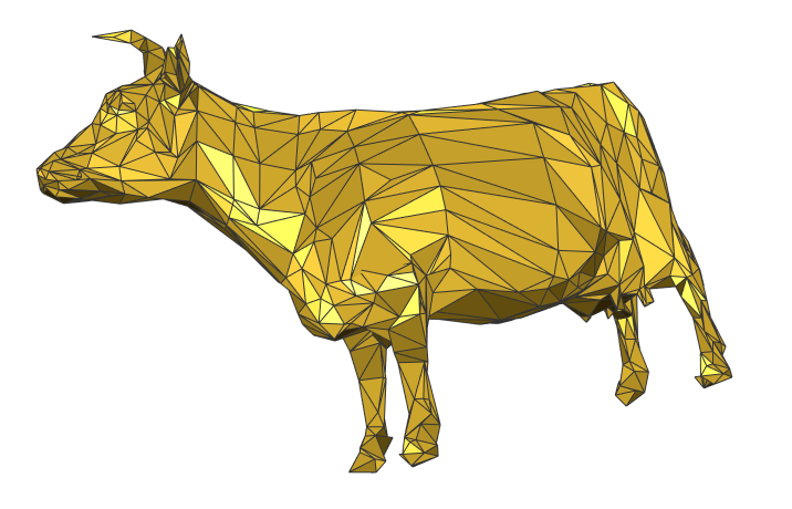
是不是很有感jio???jojo
code
https://github.com/lishaohsuai/digital_geo/tree/master/Surface_Framework_VS2017