流体模拟基础1

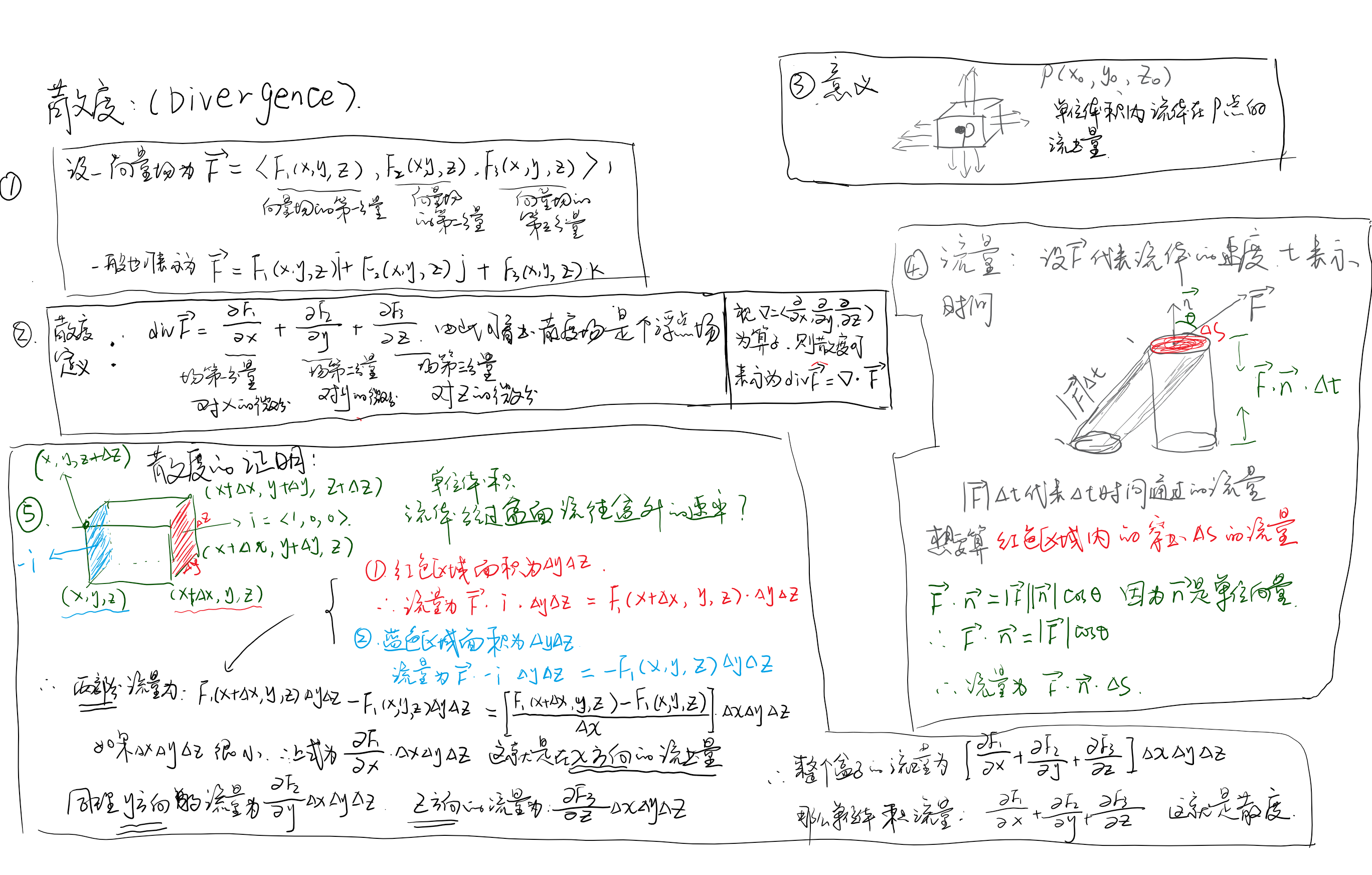
1,散度 鼠标右键打开（高清图）

 1.1 探讨1D 情况下的advection

(来自Fluid simulation for computer graphic - Robert Bridson)

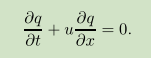
初始化一些变量:,

其中dt 按照文章写的:

import numpy as np
from matplotlib import pyplot
import time,sys

nx = 100
dx = 2/(nx-1)
nt = 100  #25 steps
u  = 1   #assume advection speed = 1
dt = dx/2


q = np.array([0.2 for x in range(nx)])

############ our init condition#######################################
# THIS CONDITION FROM PAGE-41 Robert Bridson
for x in range(2,11,1):
    q[x] = x/10.0
q[10:19] = (q[2:11])[::-1]
######################################################################

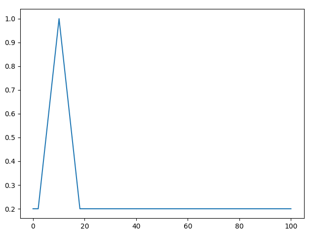
这个是初值条件:

pyplot.plot(np.linspace(0,nx,nx),q)
pyplot.show()
pyplot.close()

 接下来先用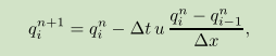 这个方法做:

def eulerian_advection():
    rhq = q.copy()  # this function compute THIS, and return this!
    qn = np.zeros(nx)
    for step in range(nt):
        # every time step we need update our READY-Q: qn
        qn = rhq.copy()
        for i in range(1,nx):
            rhq[i] = qn[i] - u * dt / dx* (qn[i] - qn[i-1])
    return rhq

pyplot.plot(np.linspace(0,nx,nx),q)
pyplot.show()
pyplot.close()

然后把这个写成人类可读的 py易读:

def eulerian_advection_very_numpy():
    rhq = q.copy()  # this function compute THIS, and return this!
    qn = np.zeros(nx)
    for step in range(nt):
        # every time step we need update our READY-Q: qn
        qn = rhq.copy()
        rhq[1:] = qn[1:] - u * dt / dx *(qn[1:] - qn[0:-1])
    return rhq
pyplot.plot(np.linspace(0,nx,nx),q)
pyplot.show()
pyplot.close()

 这个公式经过100 time step size步带来的效果,

 使用semi-lagrangian:

# fluid simulation computer graphics [page 33]
def semi_lagrangian():
    rhq = q.copy()  # this function compute THIS, and return this!
    qn = np.zeros(nx)

    for step in range(nt):
        qn = rhq.copy()

        for i in range(1, nx-1):
            xj = (i-1) * dx
            xg = i*dx
            xp = xg - dt * u
            w = (xp-xj)/dx
            qj  = qn[i-1]
            qj1 = qn[i+1]

            rhq[i] = (1-w) * qj + w * qj1
        plot_data(rhq)
    return rhq

semi_lagrangian()

 1.2 signed distance

假设速度是vector(0,1,0) 会出现下面的可视化:

2,如何在Houdini里解 2-D Linear Convection

离散完之后:

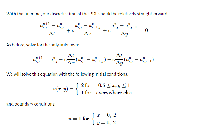
 初始条件:

Boundry地方全为0

中间设置了一些 数值.不过是把u映射到y 的高度

int row = chi("ny");
int column = chi("nx");
float c = 1;
float dx = 2.0 / float(row - 1);
float dy = 2.0 / float(column - 1);
float sigma = .2;
float dt = sigma * dx;


for(int j=0; j< row ;j++)
{
    for(int i=0; i< column ; i++)
    {
        int pt =  j * row + i;
        float u = point(0,"u",pt);
        
        // partial u/x
        int pt_x_next = j * row + i-1;
        float x_next_u = point(0,"u",pt_x_next);
        float partial_u_x = u - x_next_u;
        
        // partial u/y
        int pt_y_next = (j-1)*row + i;
        float y_next_u = point(0,"u",pt_y_next);
        float partial_u_y = u - y_next_u;
        
        
        float newu = u - c * dt/dx * ( partial_u_x) - c * dt/dy *( partial_u_y);
        setpointattrib(0,"u",pt,newu);
    }
}

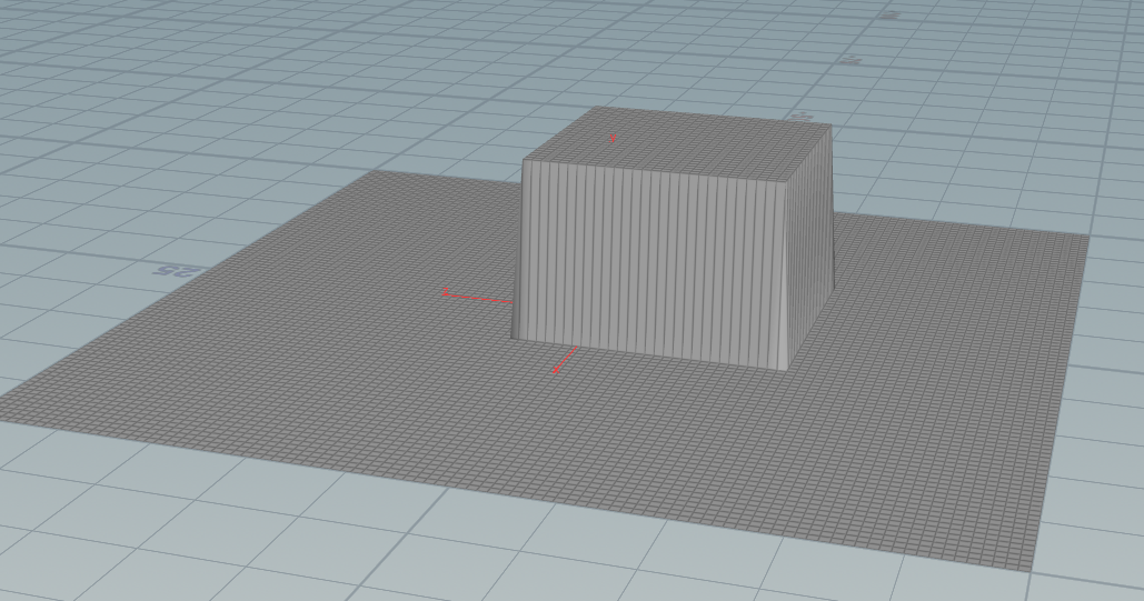
 过了一些帧

 

 Diffusion 方程:做完感觉是个高斯模糊。。。。

int row = chi("ny");
int column = chi("nx");
float c = 16;
float dx = 2.0 / float(row - 1);
float dy = 2.0 / float(column - 1);
float sigma = .05;
float dt = sigma * dx;
float viscosity = 0.05;

for(int j=1; j< row ;j++)
{
    for(int i=1; i< column ; i++)
    {
        int pt =  j * row + i;
        float u = point(0,"u",pt);
        
        
        int uxnext  = j * row + i+1;
        int uxfront = j * row + i-1;
        
        int uynext = (j+1)*row + i;
        int uyfront = (j-1)*row + i;
        
        
        // u/x 二阶偏导数
        float uxnext_val = point(0,"u",uxnext);
        float uxfront_val = point(0,"u",uxfront);
        float partial_uu_xx = uxnext_val - 2 * u + uxfront_val;
        
        // u/y 二阶偏导数
        float uynext_val = point(0,"u",uynext);
        float uyfront_val = point(0,"u",uyfront);
        float partial_uu_yy = uynext_val - 2 * u + uyfront_val;
        
 
        
        float newu = u + viscosity * dt / (dx*dx) * partial_uu_xx + viscosity*dt / (dy*dy) * partial_uu_yy ;
        
        
    
        setpointattrib(geoself(),"u",pt,newu);
    }
}

 

 第一帧:

 

过了60帧:

 

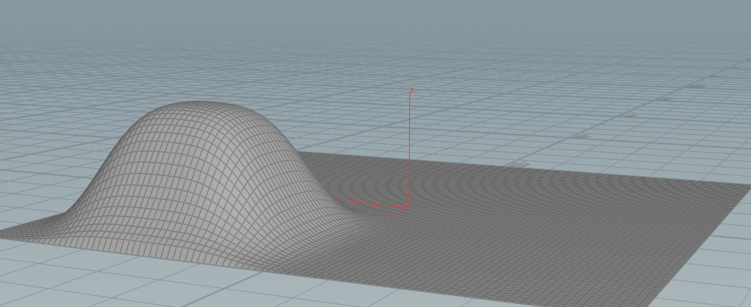
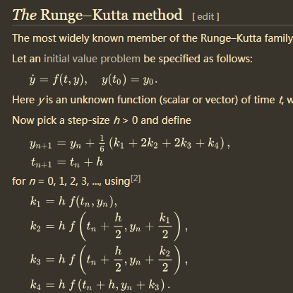
欧拉方法，K阶泰勒方法, 龙格-库塔RK2(中点midpoint), RK4

欧拉向前公式: 

欧拉向前步进法 精度测试，事实上可以用托马斯微积分给的 改进欧拉法(梯形法) 比现在这个要精确的多。

在[0,1]区间，看到n的步伐增加，对y的预测更加准确。

import numpy
from matplotlib import pyplot

def euler_step(t, y, h, yPrimFunction):
    """
    :param t: 当前时间t
    :param y: 当前值y
    :param h: 当前步长h
    :return: 时间上t+h的近似解
    """
    val =  y + h * yPrimFunction(t, y)
    return val

def euler(space, y0, n, yPrime):
    """
    :param space: [x 轴向上的区间]
    :param y0:  初值y0
    :param n:   步伐总值
    :return: [( t array) (y array)]
    """

    h = (space[1] - space[0]) / float(n)
    tArray = numpy.linspace(space[0], space[1], n)
    yArray = numpy.zeros(n)
    yArray[0] = y0
    
    for i in range(n-1):
        yArray[i+1] = euler_step(tArray[i], yArray[i], h, yPrime)
    return numpy.array((tArray,yArray))


func = lambda t, y : t * y + t*t*t
mapped_10 = euler([0, 1], 1, 10, func )
mapped_20 = euler([0, 1], 1, 20, func )
mapped_30 = euler([0, 1], 1, 30, func )
mapped_40 = euler([0, 1], 1, 40, func )

def plot_simple():
    pyplot.plot(mapped_10[0],mapped_10[1])  ##Plot the results
    pyplot.plot(mapped_20[0],mapped_20[1])  ##Plot the results
    pyplot.show()

def plot_complex():
    fig, ax = pyplot.subplots()
    ax.plot(mapped_10[0], mapped_10[1], label="n=10")
    ax.plot(mapped_20[0], mapped_20[1], label="n=20")
    ax.plot(mapped_30[0], mapped_30[1], label="n=30")
    ax.plot(mapped_40[0], mapped_40[1], label="n=40")
    ax.legend(loc=2)  # upper left corner
    ax.set_xlabel('t')
    ax.set_ylabel('y')
    ax.set_title("Euler Step method for: y'= t*y + t^3 ")
    pyplot.show()

plot_complex()

根据斜率场预测下一个值的除了欧拉法 还有几个出名的方法。

1, K阶泰勒方法 ,一阶的泰勒方法正是 欧拉方法。

    K阶的泰勒方法有个缺点，就是必须把K阶导数求出来

    围绕泰勒方法，离散方法: 求导数，ODE, PDE

    而ODE的离散方法 和 导数的离散方法，仔细观察就是从泰勒定理里 完全剥离出来的

2,但是RK2 RK3 RK4  完全是不用把不用知道 f'' f''' ... 的情况下把K阶的方法求出来，

     RK4 全局误差和h^4 成正比. 流体力学用到RK4 已经算出很高的精度了

3,还有更高级的 可变步长方法。

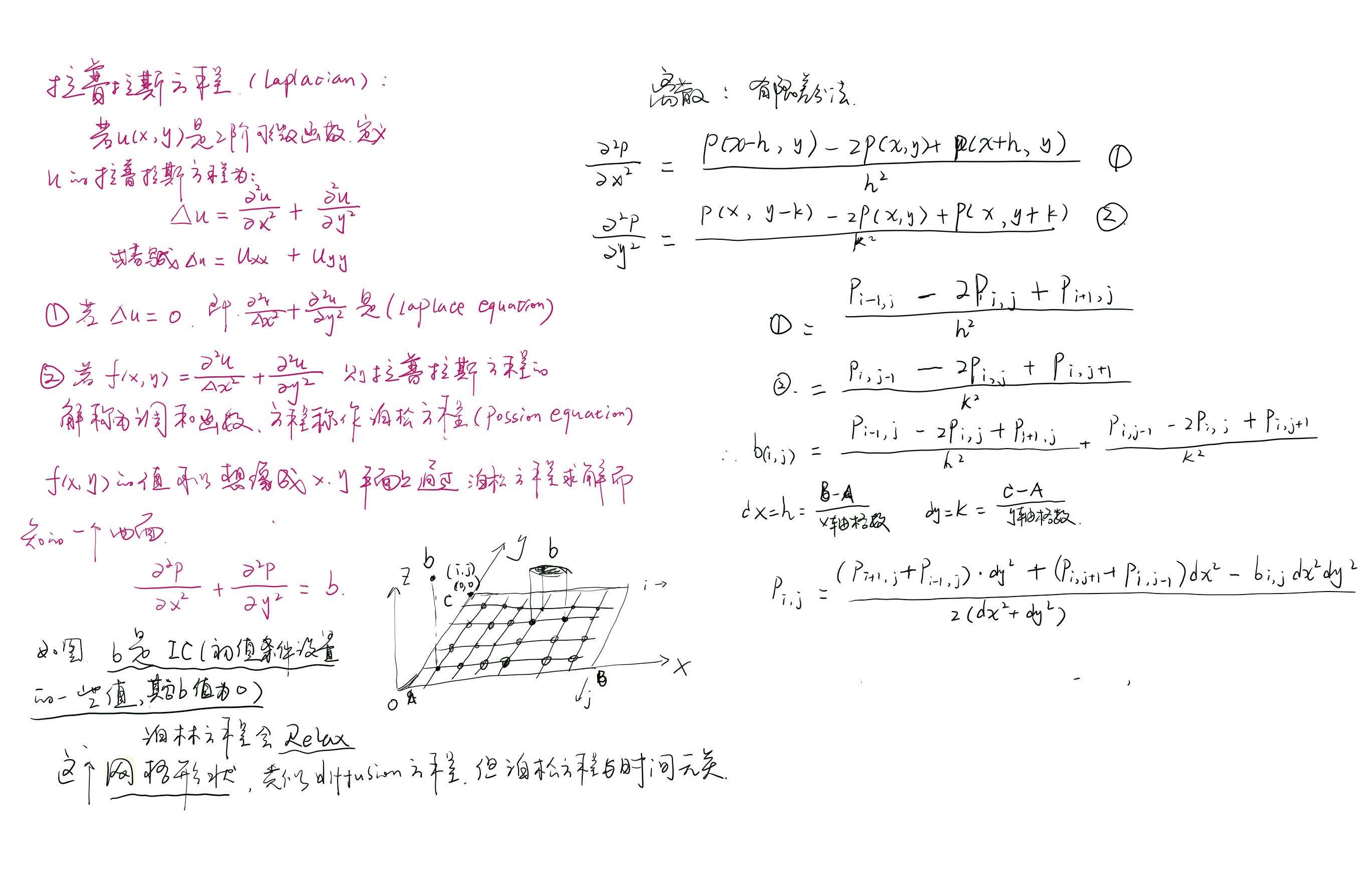
泊松方程

import numpy
from matplotlib import pyplot, cm
from mpl_toolkits.mplot3d import Axes3D

nx = 100
ny = 100

xmin = 0
xmax = 2

ymin = 0
ymax = 1

dx = (xmax - xmin) / (nx - 1)
dy = (ymax - ymin) / (ny - 1)

print(dx, dy)

p = numpy.zeros((ny, nx))
b = numpy.zeros((ny, nx))

x = numpy.linspace(xmin, xmax, nx)
y = numpy.linspace(ymin, ymax, ny)

# boundary condition for p
p[0, :] = 0  # p = 0 @ y = 1      最顶一行
p[ny - 1, :] = 0  # p = 0 @ y = 0     最底一行

p[:, 0] = 0  # p = 0 @ x = 0     左边一列
p[:, nx - 1] = 0  # p = 0 @ x = 2     右边一列

# print(p)
# init condition for b

b[:, int(ny / 2 - 10):int(ny / 2 + 10)] = 100
b[int(ny / 2 - 10):int(ny / 2 + 10):] = 100

# print(b)


square_dx = dx * dx
square_dy = dy * dy

nt = 200


def plot2D(x, y, p, frame):
    fig = pyplot.figure(figsize=(11, 7), dpi=100)
    ax = fig.gca(projection='3d')
    X, Y = numpy.meshgrid(x, y)
    surf = ax.plot_surface(X, Y, p[:], rstride=1, cstride=1, cmap=cm.viridis,
                           linewidth=0, antialiased=False)
    ax.view_init(30, 225)
    ax.set_xlabel('$x$')
    ax.set_ylabel('$y$')
    fig.savefig('./imgs/Laplace2d.' + ('00000' + str(frame))[-4:] + '.png')
    # pyplot.close()
    pyplot.show()


for it in range(nt):
    pre_p = p.copy()

    p[1:-1, 1:-1] = ((pre_p[1:-1, 2:] + pre_p[1:-1, 0:-2]) * dy * dy +
                     (pre_p[2:, 1:-1] + pre_p[:-2, 1:-1]) * dx * dx -
                     b[1:-1, 1:-1] * dx * dx * dy * dy) / (2 * (dx * dx + dy * dy))

    p[0, :] = 0  # p = 0 @ y = 1      最顶一行
    p[ny - 1, :] = 0  # p = 0 @ y = 0     最底一行
    p[:, 0] = 0  # p = 0 @ x = 0     左边一列
    p[:, nx - 1] = 0  # p = 0 @ x = 2     右边一列
    plot2D(x, y, p, it)

迭代100次的过程 

REF:

http://nbviewer.jupyter.org/github/barbagroup/CFDPython/blob/master/lessons/07_Step_5.ipynb

https://en.wikipedia.org/wiki/Euler_method

https://en.wikipedia.org/wiki/Runge%E2%80%93Kutta_methods