激活函数
激活函数----日常不能用线性方程所概括的东西
左图是线性方程,右图是非线性方程
当男生增加到一定程度的时候,喜欢女生的数量不可能无限制增加,更加趋于平稳
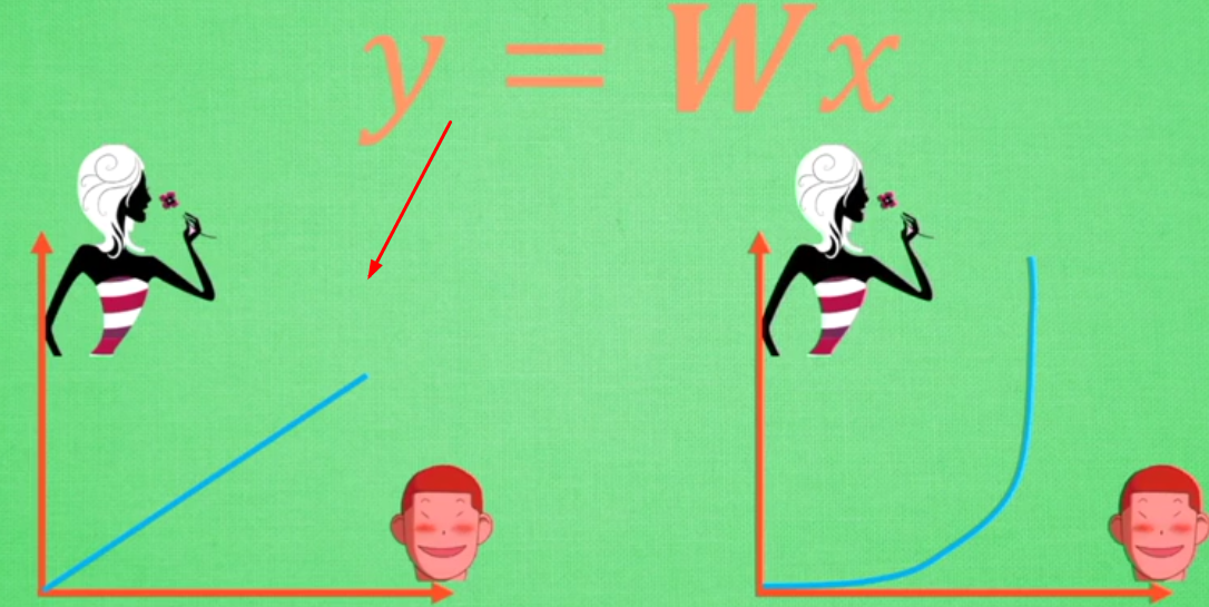
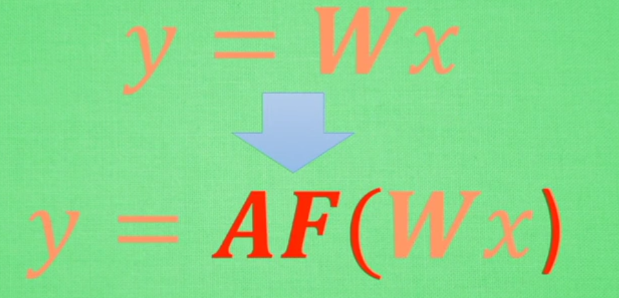
在线性基础上套了一个激活函数,使得最后能得到输出结果
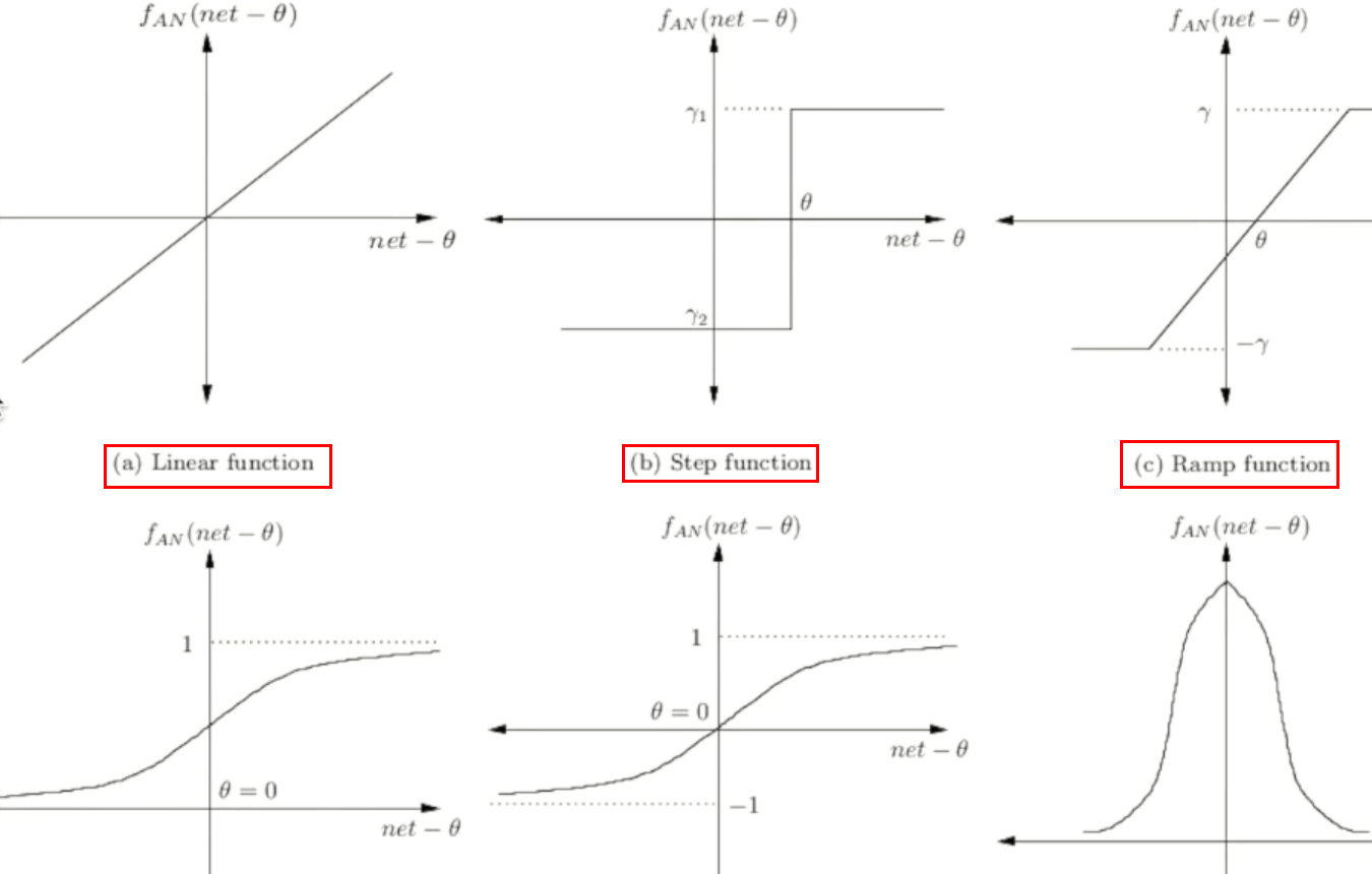
常用的三种激活函数:
取值不同时得到的结果也不同
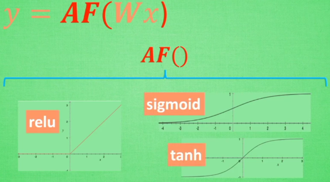
常见激活函数图形
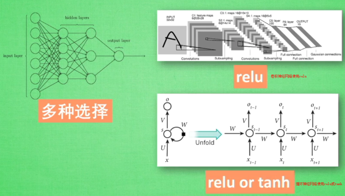
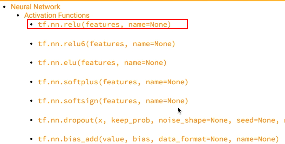
tensorflow中自带的激活函数举例:
添加隐层的神经网络
#添加隐层的神经网络结构
import tensorflow as tf

def add_layer(inputs,in_size,out_size,activation_function=None):
    #定义权重--随机生成inside和outsize的矩阵
    Weights=tf.Variable(tf.random_normal([in_size,out_size]))
    #不是矩阵,而是类似列表
    biaes=tf.Variable(tf.zeros([1,out_size])+0.1)
    Wx_plus_b=tf.matmul(inputs,Weights)+biaes
    if activation_function is  None:
        outputs=Wx_plus_b
    else:
        outputs=activation_function(Wx_plus_b)
    return outputs

import numpy as np
x_data=np.linspace(-1,1,300)[:,np.newaxis] #300行数据
noise=np.random.normal(0,0.05,x_data.shape)
y_data=np.square(x_data)-0.5+noise
#None指定sample个数,这里不限定--输出属性为1
xs=tf.placeholder(tf.float32,[None,1])  #这里需要指定tf.float32,
ys=tf.placeholder(tf.float32,[None,1])

#建造第一层layer
#输入层(1)
l1=add_layer(xs,1,10,activation_function=tf.nn.relu)
#隐层(10)
prediction=add_layer(l1,10,1,activation_function=None)
#输出层(1)
#预测prediction
loss=tf.reduce_mean(tf.reduce_sum(tf.square(ys-prediction),
                   reduction_indices=[1])) #平方误差
train_step=tf.train.GradientDescentOptimizer(0.1).minimize(loss)

init=tf.initialize_all_variables()
sess=tf.Session()
#直到执行run才执行上述操作
sess.run(init)
for i in range(1000):
    #这里假定指定所有的x_data来指定运算结果
    sess.run(train_step,feed_dict={xs:x_data,ys:y_data})
    if i%50:
        print (sess.run(loss,feed_dict={xs:x_data,ys:y_data}))
显示:
1.11593
0.26561
0.167872
0.114671
0.0835957
0.0645237
0.0524448
0.0446363
0.039476
0.0360211
0.0336599
0.0320134
0.0308378
0.0299828
0.029324
0.0287996
0.0283558
0.0279624
0.0276017
0.02726
0.0269316
0.0266103
0.026298
0.0259914
0.0256905
0.025395
0.0251055
0.0248204
0.024538
0.0242604
0.023988
0.0237211
0.0234583
0.0231979
0.0229418
0.0226901
0.0224427
0.0221994
0.0219589
0.0217222
0.0214888
0.0212535
0.0210244
0.0207988
0.0205749
0.0203548
0.0201381
增加np.newaxis
np.newaxis 为 numpy.ndarray(多维数组)增加一个轴
>> type(np.newaxis)
NoneType
>> np.newaxis == None
True
np.newaxis 在使用和功能上等价于 None,其实就是 None 的一个别名。
1. np.newaxis 的实用
>> x = np.arange(3)
>> x
array([0, 1, 2])
>> x.shape
(3,)

>> x[:, np.newaxis]
array([[0],
       [1],
       [2]])

>> x[:, None]
array([[0],
       [1],
       [2]])

>> x[:, np.newaxis].shape
 (3, 1)
2. 索引多维数组的某一列时返回的是一个行向量
>>> X = np.array([[1, 2, 3, 4], [5, 6, 7, 8], [9, 10, 11, 12]])
>>> X[:, 1]
array([2, 6, 10])       % 这里是一个行
>>> X[:, 1].shape       % X[:, 1] 的用法完全等同于一个行,而不是一个列,
(3, )
如果我们索引多维数组的某一列时,返回的仍然是列的结构,一种正确的索引方式是:
>>>X[:, 1][:, np.newaxis]
array([[2],
      [6],
      [10]])
如果想实现第二列和第四列的拼接(层叠):
>>>X_sub = np.hstack([X[:, 1][:, np.newaxis], X[:, 3][:, np.newaxis]])
                   % hstack:horizontal stack,水平方向上的层叠
>>>X_sub
array([[2, 4]
      [6, 8]
      [10, 12]])
当然更为简单的方式还是使用切片:
>> X[:, [1, 3]]
array([[ 2,  4],
       [ 6,  8],
       [10, 12]])