Stochastic Gradient Descent
https://scikit-learn.org/stable/modules/sgd.html#
随机梯度下降是一种简单且非常高效的方法, 来拟合线性分类器和回归器, 使用凸随时函数, 例如 支持向量 和 逻辑回归。
即使SGD出现在机器学习社区已经很长时间, 它才收到可观的关注量, 只在最近一些时间, 在大规模学习的场景下。
Stochastic Gradient Descent (SGD) is a simple yet very efficient approach to fitting linear classifiers and regressors under convex loss functions such as (linear) Support Vector Machines and Logistic Regression. Even though SGD has been around in the machine learning community for a long time, it has received a considerable amount of attention just recently in the context of large-scale learning.
SGD已经成功的应用于大规模和稀疏机器学习问题, 经常出现在文本分类的NLP。
如果数据是稀疏的,此模块的分类器很容器扩展到 多于10万的训练样本 和 多于10万的特征。
SGD has been successfully applied to large-scale and sparse machine learning problems often encountered in text classification and natural language processing. Given that the data is sparse, the classifiers in this module easily scale to problems with more than 10^5 training examples and more than 10^5 features.
严格地说, SGD仅仅是一种优化技术,并不对应特定的机器学习模型家族。
经常SGDClassifier 和 SGDRegressor 有一个等价的模型, 此模型不仅仅使用SGD,也使用其它的优化技术。
例如 SGDClassifier(loss='log') 产生的 逻辑回归, 即 一个模型 等价于 LogisticRegression 模型,并使用SGD, 而不是使用其它优化器(solver)。
类似地 SGDRegressor(loss='squared_loss', penalty='l2') 和 Ridge 解决相同的优化问题, 通过不同的方法。
Strictly speaking, SGD is merely an optimization technique and does not correspond to a specific family of machine learning models. It is only a way to train a model. Often, an instance of
SGDClassifierorSGDRegressorwill have an equivalent estimator in the scikit-learn API, potentially using a different optimization technique. For example, usingSGDClassifier(loss='log')results in logistic regression, i.e. a model equivalent toLogisticRegressionwhich is fitted via SGD instead of being fitted by one of the other solvers inLogisticRegression. Similarly,SGDRegressor(loss='squared_loss', penalty='l2')andRidgesolve the same optimization problem, via different means.
优点:
1 高效
2 容易实现
缺点:
1 需要大量的超参, 例如 正规化参数 和 迭代次数
2 对特征伸缩敏感
The advantages of Stochastic Gradient Descent are:
Efficiency.
Ease of implementation (lots of opportunities for code tuning).
The disadvantages of Stochastic Gradient Descent include:
SGD requires a number of hyperparameters such as the regularization parameter and the number of iterations.
SGD is sensitive to feature scaling.
Classification
SGDClassifier 类实现了普通的SGD学习规则, 支持不同的损失函数, 和 分类的惩罚项。
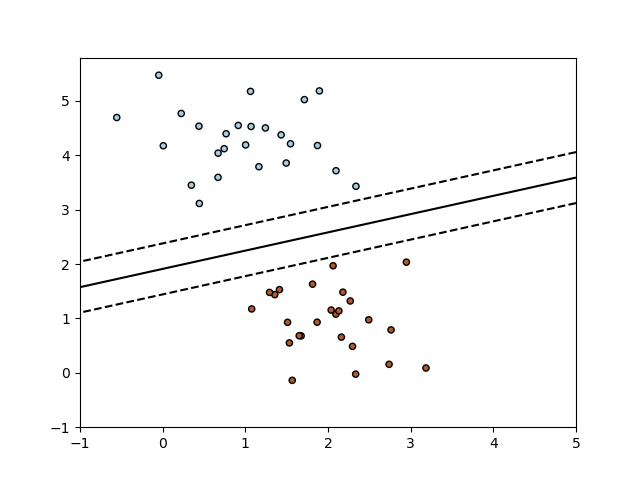
以下是 其 决策边界, 等价于 线性 SVM.
The class
SGDClassifierimplements a plain stochastic gradient descent learning routine which supports different loss functions and penalties for classification. Below is the decision boundary of aSGDClassifiertrained with the hinge loss, equivalent to a linear SVM.As other classifiers, SGD has to be fitted with two arrays: an array
Xof shape (n_samples, n_features) holding the training samples, and an array y of shape (n_samples,) holding the target values (class labels) for the training samples:

>>> from sklearn.linear_model import SGDClassifier
>>> X = [[0., 0.], [1., 1.]]
>>> y = [0, 1]
>>> clf = SGDClassifier(loss="hinge", penalty="l2", max_iter=5)
>>> clf.fit(X, y)
SGDClassifier(max_iter=5)
After being fitted, the model can then be used to predict new values:
>>> clf.predict([[2., 2.]])
array([1])
线性模型, 可以查看其对应的 系数 和 斜率。
SGD fits a linear model to the training data. The
coef_attribute holds the model parameters:
>>> clf.coef_
array([[9.9..., 9.9...]])
The
intercept_attribute holds the intercept (aka offset or bias):
>>> clf.intercept_
array([-9.9...])
距离决策平面的计算使用 decision_function
The signed distance to the hyperplane (computed as the dot product between the coefficients and the input sample, plus the intercept) is given by
SGDClassifier.decision_function:
>>> clf.decision_function([[2., 2.]])
array([29.6...])
损失函数选项
The concrete loss function can be set via the
lossparameter.SGDClassifiersupports the following loss functions:
loss="hinge": (soft-margin) linear Support Vector Machine,
loss="modified_huber": smoothed hinge loss,
loss="log": logistic regression,and all regression losses below. In this case the target is encoded as -1 or 1, and the problem is treated as a regression problem. The predicted class then correspond to the sign of the predicted target.
Regression
SGDRegressor 实现了普通的SGD学习规则, 支持不同的损失函数 和 惩罚项, 来拟合线性回归模型。
对于大量的训练样本, SGDRegressor 是非常合适的来做回归问题的解, 否则样本少的情况, 推荐使用 Ridge, Lasso, or ElasticNet
The class
SGDRegressorimplements a plain stochastic gradient descent learning routine which supports different loss functions and penalties to fit linear regression models.SGDRegressoris well suited for regression problems with a large number of training samples (> 10.000), for other problems we recommendRidge,Lasso, orElasticNet.The concrete loss function can be set via the
lossparameter.SGDRegressorsupports the following loss functions:
loss="squared_loss": Ordinary least squares,
loss="huber": Huber loss for robust regression,
loss="epsilon_insensitive": linear Support Vector Regression.
Stochastic Gradient Descent for sparse data
支持稀疏数据, 例如 文本分类中的 词 特征量。
There is built-in support for sparse data given in any matrix in a format supported by scipy.sparse. For maximum efficiency, however, use the CSR matrix format as defined in scipy.sparse.csr_matrix.
Stopping criterion
SGD提供两种停止准则, 当给定的 收敛水平达到时候。
(1)early_stopping=True,将数据集合分为 训练和 验证集合, 模型在训练结合上拟合, 停止准则基于验证集合上的预测分数。
(2)early_stopping=False, 完全基于目标函数的计算, 并运行在整个数据集合上。
The classes
SGDClassifierandSGDRegressorprovide two criteria to stop the algorithm when a given level of convergence is reached:
With
early_stopping=True, the input data is split into a training set and a validation set. The model is then fitted on the training set, and the stopping criterion is based on the prediction score (using thescoremethod) computed on the validation set. The size of the validation set can be changed with the parametervalidation_fraction.With
early_stopping=False, the model is fitted on the entire input data and the stopping criterion is based on the objective function computed on the training data.
SGDClassifier
https://scikit-learn.org/stable/modules/generated/sklearn.linear_model.SGDClassifier.html#sklearn.linear_model.SGDClassifier.fit
SGD支持在线学习, minibatch。
Linear classifiers (SVM, logistic regression, etc.) with SGD training.
This estimator implements regularized linear models with stochastic gradient descent (SGD) learning: the gradient of the loss is estimated each sample at a time and the model is updated along the way with a decreasing strength schedule (aka learning rate). SGD allows minibatch (online/out-of-core) learning via the
partial_fitmethod. For best results using the default learning rate schedule, the data should have zero mean and unit variance.This implementation works with data represented as dense or sparse arrays of floating point values for the features. The model it fits can be controlled with the loss parameter; by default, it fits a linear support vector machine (SVM).
The regularizer is a penalty added to the loss function that shrinks model parameters towards the zero vector using either the squared euclidean norm L2 or the absolute norm L1 or a combination of both (Elastic Net). If the parameter update crosses the 0.0 value because of the regularizer, the update is truncated to 0.0 to allow for learning sparse models and achieve online feature selection.
>>> import numpy as np
>>> from sklearn.linear_model import SGDClassifier
>>> from sklearn.preprocessing import StandardScaler
>>> from sklearn.pipeline import make_pipeline
>>> X = np.array([[-1, -1], [-2, -1], [1, 1], [2, 1]])
>>> Y = np.array([1, 1, 2, 2])
>>> # Always scale the input. The most convenient way is to use a pipeline.
>>> clf = make_pipeline(StandardScaler(),
...                     SGDClassifier(max_iter=1000, tol=1e-3))
>>> clf.fit(X, Y)
Pipeline(steps=[('standardscaler', StandardScaler()),
                ('sgdclassifier', SGDClassifier())])
>>> print(clf.predict([[-0.8, -1]]))
[1]
SGD: Maximum margin separating hyperplane
https://scikit-learn.org/stable/auto_examples/linear_model/plot_sgd_separating_hyperplane.html#sphx-glr-auto-examples-linear-model-plot-sgd-separating-hyperplane-py
构造二值可分数据,使用SGD算法训练模型, 使用contour绘制分离边际的超平面。
Plot the maximum margin separating hyperplane within a two-class separable dataset using a linear Support Vector Machines classifier trained using SGD.
print(__doc__)

import numpy as np
import matplotlib.pyplot as plt
from sklearn.linear_model import SGDClassifier
from sklearn.datasets import make_blobs

# we create 50 separable points
X, Y = make_blobs(n_samples=50, centers=2, random_state=0, cluster_std=0.60)

# fit the model
clf = SGDClassifier(loss="hinge", alpha=0.01, max_iter=200)

clf.fit(X, Y)

# plot the line, the points, and the nearest vectors to the plane
xx = np.linspace(-1, 5, 10)
yy = np.linspace(-1, 5, 10)

X1, X2 = np.meshgrid(xx, yy)
Z = np.empty(X1.shape)
for (i, j), val in np.ndenumerate(X1):
    x1 = val
    x2 = X2[i, j]
    p = clf.decision_function([[x1, x2]])
    Z[i, j] = p[0]
levels = [-1.0, 0.0, 1.0]
linestyles = ['dashed', 'solid', 'dashed']
colors = 'k'
plt.contour(X1, X2, Z, levels, colors=colors, linestyles=linestyles)
plt.scatter(X[:, 0], X[:, 1], c=Y, cmap=plt.cm.Paired,
            edgecolor='black', s=20)

plt.axis('tight')
plt.show()
Classification of text documents using sparse features
https://scikit-learn.org/stable/auto_examples/text/plot_document_classification_20newsgroups.html#sphx-glr-auto-examples-text-plot-document-classification-20newsgroups-py
对于稀疏数据, 以下模型展示了其性能。
可知: 在同等分值情况下, 贝叶斯模型耗时最短, SGD也不错。
This is an example showing how scikit-learn can be used to classify documents by topics using a bag-of-words approach. This example uses a scipy.sparse matrix to store the features and demonstrates various classifiers that can efficiently handle sparse matrices.

"""
======================================================
Classification of text documents using sparse features
======================================================

This is an example showing how scikit-learn can be used to classify documents
by topics using a bag-of-words approach. This example uses a scipy.sparse
matrix to store the features and demonstrates various classifiers that can
efficiently handle sparse matrices.

The dataset used in this example is the 20 newsgroups dataset. It will be
automatically downloaded, then cached.

"""

# Author: Peter Prettenhofer <peter.prettenhofer@gmail.com>
#         Olivier Grisel <olivier.grisel@ensta.org>
#         Mathieu Blondel <mathieu@mblondel.org>
#         Lars Buitinck
# License: BSD 3 clause
import logging
import numpy as np
from optparse import OptionParser
import sys
from time import time
import matplotlib.pyplot as plt

from sklearn.datasets import fetch_20newsgroups
from sklearn.feature_extraction.text import TfidfVectorizer
from sklearn.feature_extraction.text import HashingVectorizer
from sklearn.feature_selection import SelectFromModel
from sklearn.feature_selection import SelectKBest, chi2
from sklearn.linear_model import RidgeClassifier
from sklearn.pipeline import Pipeline
from sklearn.svm import LinearSVC
from sklearn.linear_model import SGDClassifier
from sklearn.linear_model import Perceptron
from sklearn.linear_model import PassiveAggressiveClassifier
from sklearn.naive_bayes import BernoulliNB, ComplementNB, MultinomialNB
from sklearn.neighbors import KNeighborsClassifier
from sklearn.neighbors import NearestCentroid
from sklearn.ensemble import RandomForestClassifier
from sklearn.utils.extmath import density
from sklearn import metrics


# Display progress logs on stdout
logging.basicConfig(level=logging.INFO,
                    format='%(asctime)s %(levelname)s %(message)s')

op = OptionParser()
op.add_option("--report",
              action="store_true", dest="print_report",
              help="Print a detailed classification report.")
op.add_option("--chi2_select",
              action="store", type="int", dest="select_chi2",
              help="Select some number of features using a chi-squared test")
op.add_option("--confusion_matrix",
              action="store_true", dest="print_cm",
              help="Print the confusion matrix.")
op.add_option("--top10",
              action="store_true", dest="print_top10",
              help="Print ten most discriminative terms per class"
                   " for every classifier.")
op.add_option("--all_categories",
              action="store_true", dest="all_categories",
              help="Whether to use all categories or not.")
op.add_option("--use_hashing",
              action="store_true",
              help="Use a hashing vectorizer.")
op.add_option("--n_features",
              action="store", type=int, default=2 ** 16,
              help="n_features when using the hashing vectorizer.")
op.add_option("--filtered",
              action="store_true",
              help="Remove newsgroup information that is easily overfit: "
                   "headers, signatures, and quoting.")


def is_interactive():
    return not hasattr(sys.modules['__main__'], '__file__')


# work-around for Jupyter notebook and IPython console
argv = [] if is_interactive() else sys.argv[1:]
(opts, args) = op.parse_args(argv)
if len(args) > 0:
    op.error("this script takes no arguments.")
    sys.exit(1)

print(__doc__)
op.print_help()
print()


# %%
# Load data from the training set
# ------------------------------------
# Let's load data from the newsgroups dataset which comprises around 18000
# newsgroups posts on 20 topics split in two subsets: one for training (or
# development) and the other one for testing (or for performance evaluation).
if opts.all_categories:
    categories = None
else:
    categories = [
        'alt.atheism',
        'talk.religion.misc',
        'comp.graphics',
        'sci.space',
    ]

if opts.filtered:
    remove = ('headers', 'footers', 'quotes')
else:
    remove = ()

print("Loading 20 newsgroups dataset for categories:")
print(categories if categories else "all")

data_train = fetch_20newsgroups(subset='train', categories=categories,
                                shuffle=True, random_state=42,
                                remove=remove)

data_test = fetch_20newsgroups(subset='test', categories=categories,
                               shuffle=True, random_state=42,
                               remove=remove)
print('data loaded')

# order of labels in `target_names` can be different from `categories`
target_names = data_train.target_names


def size_mb(docs):
    return sum(len(s.encode('utf-8')) for s in docs) / 1e6


data_train_size_mb = size_mb(data_train.data)
data_test_size_mb = size_mb(data_test.data)

print("%d documents - %0.3fMB (training set)" % (
    len(data_train.data), data_train_size_mb))
print("%d documents - %0.3fMB (test set)" % (
    len(data_test.data), data_test_size_mb))
print("%d categories" % len(target_names))
print()

# split a training set and a test set
y_train, y_test = data_train.target, data_test.target

print("Extracting features from the training data using a sparse vectorizer")
t0 = time()
if opts.use_hashing:
    vectorizer = HashingVectorizer(stop_words='english', alternate_sign=False,
                                   n_features=opts.n_features)
    X_train = vectorizer.transform(data_train.data)
else:
    vectorizer = TfidfVectorizer(sublinear_tf=True, max_df=0.5,
                                 stop_words='english')
    X_train = vectorizer.fit_transform(data_train.data)
duration = time() - t0
print("done in %fs at %0.3fMB/s" % (duration, data_train_size_mb / duration))
print("n_samples: %d, n_features: %d" % X_train.shape)
print()

print("Extracting features from the test data using the same vectorizer")
t0 = time()
X_test = vectorizer.transform(data_test.data)
duration = time() - t0
print("done in %fs at %0.3fMB/s" % (duration, data_test_size_mb / duration))
print("n_samples: %d, n_features: %d" % X_test.shape)
print()

# mapping from integer feature name to original token string
if opts.use_hashing:
    feature_names = None
else:
    feature_names = vectorizer.get_feature_names()

if opts.select_chi2:
    print("Extracting %d best features by a chi-squared test" %
          opts.select_chi2)
    t0 = time()
    ch2 = SelectKBest(chi2, k=opts.select_chi2)
    X_train = ch2.fit_transform(X_train, y_train)
    X_test = ch2.transform(X_test)
    if feature_names:
        # keep selected feature names
        feature_names = [feature_names[i] for i
                         in ch2.get_support(indices=True)]
    print("done in %fs" % (time() - t0))
    print()

if feature_names:
    feature_names = np.asarray(feature_names)


def trim(s):
    """Trim string to fit on terminal (assuming 80-column display)"""
    return s if len(s) <= 80 else s[:77] + "..."


# %%
# Benchmark classifiers
# ------------------------------------
# We train and test the datasets with 15 different classification models
# and get performance results for each model.
def benchmark(clf):
    print('_' * 80)
    print("Training: ")
    print(clf)
    t0 = time()
    clf.fit(X_train, y_train)
    train_time = time() - t0
    print("train time: %0.3fs" % train_time)

    t0 = time()
    pred = clf.predict(X_test)
    test_time = time() - t0
    print("test time:  %0.3fs" % test_time)

    score = metrics.accuracy_score(y_test, pred)
    print("accuracy:   %0.3f" % score)

    if hasattr(clf, 'coef_'):
        print("dimensionality: %d" % clf.coef_.shape[1])
        print("density: %f" % density(clf.coef_))

        if opts.print_top10 and feature_names is not None:
            print("top 10 keywords per class:")
            for i, label in enumerate(target_names):
                top10 = np.argsort(clf.coef_[i])[-10:]
                print(trim("%s: %s" % (label, " ".join(feature_names[top10]))))
        print()

    if opts.print_report:
        print("classification report:")
        print(metrics.classification_report(y_test, pred,
                                            target_names=target_names))

    if opts.print_cm:
        print("confusion matrix:")
        print(metrics.confusion_matrix(y_test, pred))

    print()
    clf_descr = str(clf).split('(')[0]
    return clf_descr, score, train_time, test_time


results = []
for clf, name in (
        (RidgeClassifier(tol=1e-2, solver="sag"), "Ridge Classifier"),
        (Perceptron(max_iter=50), "Perceptron"),
        (PassiveAggressiveClassifier(max_iter=50),
         "Passive-Aggressive"),
        (KNeighborsClassifier(n_neighbors=10), "kNN"),
        (RandomForestClassifier(), "Random forest")):
    print('=' * 80)
    print(name)
    results.append(benchmark(clf))

for penalty in ["l2", "l1"]:
    print('=' * 80)
    print("%s penalty" % penalty.upper())
    # Train Liblinear model
    results.append(benchmark(LinearSVC(penalty=penalty, dual=False,
                                       tol=1e-3)))

    # Train SGD model
    results.append(benchmark(SGDClassifier(alpha=.0001, max_iter=50,
                                           penalty=penalty)))

# Train SGD with Elastic Net penalty
print('=' * 80)
print("Elastic-Net penalty")
results.append(benchmark(SGDClassifier(alpha=.0001, max_iter=50,
                                       penalty="elasticnet")))

# Train NearestCentroid without threshold
print('=' * 80)
print("NearestCentroid (aka Rocchio classifier)")
results.append(benchmark(NearestCentroid()))

# Train sparse Naive Bayes classifiers
print('=' * 80)
print("Naive Bayes")
results.append(benchmark(MultinomialNB(alpha=.01)))
results.append(benchmark(BernoulliNB(alpha=.01)))
results.append(benchmark(ComplementNB(alpha=.1)))

print('=' * 80)
print("LinearSVC with L1-based feature selection")
# The smaller C, the stronger the regularization.
# The more regularization, the more sparsity.
results.append(benchmark(Pipeline([
  ('feature_selection', SelectFromModel(LinearSVC(penalty="l1", dual=False,
                                                  tol=1e-3))),
  ('classification', LinearSVC(penalty="l2"))])))


# %%
# Add plots
# ------------------------------------
# The bar plot indicates the accuracy, training time (normalized) and test time
# (normalized) of each classifier.
indices = np.arange(len(results))

results = [[x[i] for x in results] for i in range(4)]

clf_names, score, training_time, test_time = results
training_time = np.array(training_time) / np.max(training_time)
test_time = np.array(test_time) / np.max(test_time)

plt.figure(figsize=(12, 8))
plt.title("Score")
plt.barh(indices, score, .2, label="score", color='navy')
plt.barh(indices + .3, training_time, .2, label="training time",
         color='c')
plt.barh(indices + .6, test_time, .2, label="test time", color='darkorange')
plt.yticks(())
plt.legend(loc='best')
plt.subplots_adjust(left=.25)
plt.subplots_adjust(top=.95)
plt.subplots_adjust(bottom=.05)

for i, c in zip(indices, clf_names):
    plt.text(-.3, i, c)

plt.show()
SVM: Separating hyperplane for unbalanced classes
https://scikit-learn.org/stable/auto_examples/svm/plot_separating_hyperplane_unbalanced.html#sphx-glr-auto-examples-svm-plot-separating-hyperplane-unbalanced-py
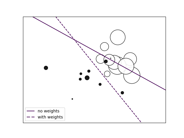
对于分类样本不均衡的情况, 使用SVC线性模型, 可以设置 class_weight 对数据量少的分类数据进行 强化。
然后通过contour图展示 两种情况的 分类平面。
如果不添加 class_weight 参数, 则会牺牲少数类别的 分类结果,
添加后, 会保证少数类别的分类质量。
Find the optimal separating hyperplane using an SVC for classes that are unbalanced.
We first find the separating plane with a plain SVC and then plot (dashed) the separating hyperplane with automatically correction for unbalanced classes.

print(__doc__)

import numpy as np
import matplotlib.pyplot as plt
from sklearn import svm
from sklearn.datasets import make_blobs

# we create two clusters of random points
n_samples_1 = 1000
n_samples_2 = 100
centers = [[0.0, 0.0], [2.0, 2.0]]
clusters_std = [1.5, 0.5]
X, y = make_blobs(n_samples=[n_samples_1, n_samples_2],
                  centers=centers,
                  cluster_std=clusters_std,
                  random_state=0, shuffle=False)

# fit the model and get the separating hyperplane
clf = svm.SVC(kernel='linear', C=1.0)
clf.fit(X, y)

# fit the model and get the separating hyperplane using weighted classes
wclf = svm.SVC(kernel='linear', class_weight={1: 10})
wclf.fit(X, y)

# plot the samples
plt.scatter(X[:, 0], X[:, 1], c=y, cmap=plt.cm.Paired, edgecolors='k')

# plot the decision functions for both classifiers
ax = plt.gca()
xlim = ax.get_xlim()
ylim = ax.get_ylim()

# create grid to evaluate model
xx = np.linspace(xlim[0], xlim[1], 30)
yy = np.linspace(ylim[0], ylim[1], 30)
YY, XX = np.meshgrid(yy, xx)
xy = np.vstack([XX.ravel(), YY.ravel()]).T

# get the separating hyperplane
Z = clf.decision_function(xy).reshape(XX.shape)

# plot decision boundary and margins
a = ax.contour(XX, YY, Z, colors='k', levels=[0], alpha=0.5, linestyles=['-'])

# get the separating hyperplane for weighted classes
Z = wclf.decision_function(xy).reshape(XX.shape)

# plot decision boundary and margins for weighted classes
b = ax.contour(XX, YY, Z, colors='r', levels=[0], alpha=0.5, linestyles=['-'])

plt.legend([a.collections[0], b.collections[0]], ["non weighted", "weighted"],
           loc="upper right")
plt.show()
Comparing various online solvers
https://scikit-learn.org/stable/auto_examples/linear_model/plot_sgd_comparison.html#sphx-glr-auto-examples-linear-model-plot-sgd-comparison-py
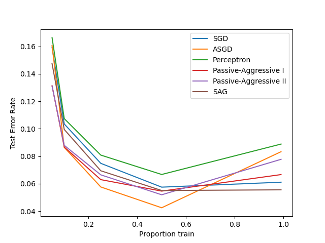
展示不同在线优化器在手写识别数据上的性能。
以 训练集合 的依次递增为横坐标。
以 验证集合 的测试错误率为纵坐标。
ASGD性能最好。
An example showing how different online solvers perform on the hand-written digits dataset.
Out:
training SGD
training ASGD
training Perceptron
training Passive-Aggressive I
training Passive-Aggressive II
training SAG
# Author: Rob Zinkov <rob at zinkov dot com>
# License: BSD 3 clause

import numpy as np
import matplotlib.pyplot as plt
from sklearn import datasets

from sklearn.model_selection import train_test_split
from sklearn.linear_model import SGDClassifier, Perceptron
from sklearn.linear_model import PassiveAggressiveClassifier
from sklearn.linear_model import LogisticRegression

heldout = [0.95, 0.90, 0.75, 0.50, 0.01]
rounds = 20
X, y = datasets.load_digits(return_X_y=True)

classifiers = [
    ("SGD", SGDClassifier(max_iter=100)),
    ("ASGD", SGDClassifier(average=True)),
    ("Perceptron", Perceptron()),
    ("Passive-Aggressive I", PassiveAggressiveClassifier(loss='hinge',
                                                         C=1.0, tol=1e-4)),
    ("Passive-Aggressive II", PassiveAggressiveClassifier(loss='squared_hinge',
                                                          C=1.0, tol=1e-4)),
    ("SAG", LogisticRegression(solver='sag', tol=1e-1, C=1.e4 / X.shape[0]))
]

xx = 1. - np.array(heldout)

for name, clf in classifiers:
    print("training %s" % name)
    rng = np.random.RandomState(42)
    yy = []
    for i in heldout:
        yy_ = []
        for r in range(rounds):
            X_train, X_test, y_train, y_test =
                train_test_split(X, y, test_size=i, random_state=rng)
            clf.fit(X_train, y_train)
            y_pred = clf.predict(X_test)
            yy_.append(1 - np.mean(y_pred == y_test))
        yy.append(np.mean(yy_))
    plt.plot(xx, yy, label=name)

plt.legend(loc="upper right")
plt.xlabel("Proportion train")
plt.ylabel("Test Error Rate")
plt.show()
train_test_split
https://scikit-learn.org/stable/modules/generated/sklearn.model_selection.train_test_split.html#sklearn.model_selection.train_test_split
使用 test_size 参数划分 训练和验证集合的大小。
Split arrays or matrices into random train and test subsets
Quick utility that wraps input validation and
next(ShuffleSplit().split(X, y))and application to input data into a single call for splitting (and optionally subsampling) data in a oneliner.
>>> X_train, X_test, y_train, y_test = train_test_split(
...     X, y, test_size=0.33, random_state=42)
...
>>> X_train
array([[4, 5],
       [0, 1],
       [6, 7]])
>>> y_train
[2, 0, 3]
>>> X_test
array([[2, 3],
       [8, 9]])
>>> y_test
[1, 4]
SGD: Weighted samples
https://scikit-learn.org/stable/auto_examples/linear_model/plot_sgd_weighted_samples.html#sphx-glr-auto-examples-linear-model-plot-sgd-weighted-samples-py
对于特别要关注的训练数据, 可以通过 sample_weight 来强化其在模型训练中的影响。
与 class_weight 不同, 其更加灵活, 可以对具体的模型数据进行强化。
如下示例, 经过强化后的数据的分类正确率 得到了保障。
Plot decision function of a weighted dataset, where the size of points is proportional to its weight.
print(__doc__)

import numpy as np
import matplotlib.pyplot as plt
from sklearn import linear_model

# we create 20 points
np.random.seed(0)
X = np.r_[np.random.randn(10, 2) + [1, 1], np.random.randn(10, 2)]
y = [1] * 10 + [-1] * 10
sample_weight = 100 * np.abs(np.random.randn(20))
# and assign a bigger weight to the last 10 samples
sample_weight[:10] *= 10

# plot the weighted data points
xx, yy = np.meshgrid(np.linspace(-4, 5, 500), np.linspace(-4, 5, 500))
plt.figure()
plt.scatter(X[:, 0], X[:, 1], c=y, s=sample_weight, alpha=0.9,
            cmap=plt.cm.bone, edgecolor='black')

# fit the unweighted model
clf = linear_model.SGDClassifier(alpha=0.01, max_iter=100)
clf.fit(X, y)
Z = clf.decision_function(np.c_[xx.ravel(), yy.ravel()])
Z = Z.reshape(xx.shape)
no_weights = plt.contour(xx, yy, Z, levels=[0], linestyles=['solid'])

# fit the weighted model
clf = linear_model.SGDClassifier(alpha=0.01, max_iter=100)
clf.fit(X, y, sample_weight=sample_weight)
Z = clf.decision_function(np.c_[xx.ravel(), yy.ravel()])
Z = Z.reshape(xx.shape)
samples_weights = plt.contour(xx, yy, Z, levels=[0], linestyles=['dashed'])

plt.legend([no_weights.collections[0], samples_weights.collections[0]],
           ["no weights", "with weights"], loc="lower left")

plt.xticks(())
plt.yticks(())
plt.show()
Python Numpy模块函数np.c_和np.r_
https://www.cnblogs.com/shaosks/p/9890787.html
按列拼接,或者 按行拼接。
np.r_:是按列连接两个矩阵,就是把两矩阵上下相加,要求列数相等,类似于pandas中的concat()。
np.c_:是按行连接两个矩阵,就是把两矩阵左右相加,要求行数相等,类似于pandas中的merge()。
复制代码

import numpy as np
a = np.array([1, 2, 3])
b = np.array([4, 5, 6])
c = np.c_[a,b]

print(np.r_[a,b])
print('
')
print(c)
print('
')
print(np.c_[c,a])
################################
结果:
[1 2 3 4 5 6]


[[1 4]
 [2 5]
 [3 6]]


[[1 4 1]
 [2 5 2]
 [3 6 3]]
https://numpy.org/doc/stable/reference/generated/numpy.r_.html
分类问题-样本权重(sample_weight)和类别权重(class_weight)
https://zhuanlan.zhihu.com/p/75679299
- 类型权重参数: class_weight
class_weight有什么作用?在分类模型中,我们经常会遇到两类问题:
第一种是误分类的代价很高。比如对合法用户和非法用户进行分类,将非法用户分类为合法用户的代价很高,我们宁愿将合法用户分类为非法用户,这时可以人工再甄别,但是却不愿将非法用户分类为合法用户。这时,我们可以适当提高非法用户的权重class_weight={0:0.9, 1:0.1}。
第二种是样本是高度失衡的,比如我们有合法用户和非法用户的二元样本数据10000条,里面合法用户有9995条,非法用户只有5条,如果我们不考虑权重,则我们可以将所有的测试集都预测为合法用户,这样预测准确率理论上有99.95%,但是却没有任何意义。这时,我们可以选择balanced(scikit-learn 逻辑回归类库使用小结),让类库自动提高非法用户样本的权重。
2. 样本权重参数: sample_weight
样本不平衡,导致样本不是总体样本的无偏估计,从而可能导致我们的模型预测能力下降。遇到这种情况,我们可以通过调节样本权重来尝试解决这个问题。调节样本权重的方法有两种,第一种是在class_weight使用balanced。第二种是在调用fit函数时,通过sample_weight来自己调节每个样本权重。
在scikit-learn做逻辑回归时,如果上面两种方法都用到了,那么样本的真正权重是class_weight*sample_weight.
Plot multi-class SGD on the iris dataset
https://scikit-learn.org/stable/auto_examples/linear_model/plot_sgd_iris.html#sphx-glr-auto-examples-linear-model-plot-sgd-iris-py
多分类问题, 绘制超平面 和 contour图。
Plot decision surface of multi-class SGD on iris dataset. The hyperplanes corresponding to the three one-versus-all (OVA) classifiers are represented by the dashed lines.
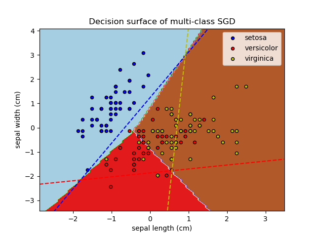
print(__doc__)

import numpy as np
import matplotlib.pyplot as plt
from sklearn import datasets
from sklearn.linear_model import SGDClassifier

# import some data to play with
iris = datasets.load_iris()

# we only take the first two features. We could
# avoid this ugly slicing by using a two-dim dataset
X = iris.data[:, :2]
y = iris.target
colors = "bry"

# shuffle
idx = np.arange(X.shape[0])
np.random.seed(13)
np.random.shuffle(idx)
X = X[idx]
y = y[idx]

# standardize
mean = X.mean(axis=0)
std = X.std(axis=0)
X = (X - mean) / std

h = .02  # step size in the mesh

clf = SGDClassifier(alpha=0.001, max_iter=100).fit(X, y)

# create a mesh to plot in
x_min, x_max = X[:, 0].min() - 1, X[:, 0].max() + 1
y_min, y_max = X[:, 1].min() - 1, X[:, 1].max() + 1
xx, yy = np.meshgrid(np.arange(x_min, x_max, h),
                     np.arange(y_min, y_max, h))

# Plot the decision boundary. For that, we will assign a color to each
# point in the mesh [x_min, x_max]x[y_min, y_max].
Z = clf.predict(np.c_[xx.ravel(), yy.ravel()])
# Put the result into a color plot
Z = Z.reshape(xx.shape)
cs = plt.contourf(xx, yy, Z, cmap=plt.cm.Paired)
plt.axis('tight')

# Plot also the training points
for i, color in zip(clf.classes_, colors):
    idx = np.where(y == i)
    plt.scatter(X[idx, 0], X[idx, 1], c=color, label=iris.target_names[i],
                cmap=plt.cm.Paired, edgecolor='black', s=20)
plt.title("Decision surface of multi-class SGD")
plt.axis('tight')

# Plot the three one-against-all classifiers
xmin, xmax = plt.xlim()
ymin, ymax = plt.ylim()
coef = clf.coef_
intercept = clf.intercept_


def plot_hyperplane(c, color):
    def line(x0):
        return (-(x0 * coef[c, 0]) - intercept[c]) / coef[c, 1]

    plt.plot([xmin, xmax], [line(xmin), line(xmax)],
             ls="--", color=color)


for i, color in zip(clf.classes_, colors):
    plot_hyperplane(i, color)
plt.legend()
plt.show()
numpy.where
https://numpy.org/doc/stable/reference/generated/numpy.where.html#numpy.where
numpy.where(condition[, x, y])Return elements chosen from x or y depending on condition.
Note
When only condition is provided, this function is a shorthand for
np.asarray(condition).nonzero(). Usingnonzerodirectly should be preferred, as it behaves correctly for subclasses. The rest of this documentation covers only the case where all three arguments are provided.
- Parameters
- conditionarray_like, bool
Where True, yield x, otherwise yield y.
- x, yarray_like
Values from which to choose. x, y and condition need to be broadcastable to some shape.
- Returns
- outndarray
An array with elements from x where condition is True, and elements from y elsewhere.
a = np.arange(10)

a
array([0, 1, 2, 3, 4, 5, 6, 7, 8, 9])

np.where(a < 5, a, 10*a)
array([ 0,  1,  2,  3,  4, 50, 60, 70, 80, 90])
a = np.asarray([3, 2, 1])
a
Out[15]: array([3, 2, 1])
np.where(a == 1)
Out[16]: (array([2], dtype=int64),)
a == 1
Out[17]: array([False, False,  True])
用梯度下降解决回归问题
https://paradiseeee.github.io/2019/03/02/Python-DataScience-CookBook-Learning-Notes-(III)/