-
什么品牌的手机最受欢迎?
-
这些手机的平均价格、最高价格、最低价格?
-
这些手机每月的销售情况如何?
实现这些统计功能的比数据库的sql要方便的多,而且查询速度非常快,可以实现实时搜索效果。
Elasticsearch中的聚合,包含多种类型,最常用的两种,一个叫桶,一个叫度量:
桶(bucket)
桶的作用,是按照某种方式对数据进行分组,每一组数据在ES中称为一个桶,例如我们根据国籍对人划分,可以得到中国桶、英国桶,日本桶……或者我们按照年龄段对人进行划分:0~10,10~20,20~30,30~40等。
Elasticsearch中提供的划分桶的方式有很多:
-
Date Histogram Aggregation:根据日期阶梯分组,例如给定阶梯为周,会自动每周分为一组
-
Histogram Aggregation:根据数值阶梯分组,与日期类似
-
Terms Aggregation:根据词条内容分组,词条内容完全匹配的为一组
-
Range Aggregation:数值和日期的范围分组,指定开始和结束,然后按段分组
bucket aggregations 只负责对数据进行分组,并不进行计算,因此往往bucket中往往会嵌套另一种聚合:metrics aggregations即度量
度量(metrics)
分组完成以后,我们一般会对组中的数据进行聚合运算,例如求平均值、最大、最小、求和等,这些在ES中称为度量
比较常用的一些度量聚合方式:
-
Avg Aggregation:求平均值
-
Max Aggregation:求最大值
-
Min Aggregation:求最小值
-
Percentiles Aggregation:求百分比
-
Stats Aggregation:同时返回avg、max、min、sum、count等
-
Sum Aggregation:求和
-
Top hits Aggregation:求前几
-
Value Count Aggregation:求总数
-
……
为了测试聚合,我们先批量导入一些数据
创建索引
PUT /cars
{
  "settings": {
    "number_of_shards": 1,
    "number_of_replicas": 0
  },
  "mappings": {
    "transactions": {
      "properties": {
        "color": {
          "type": "keyword"
        },
        "make": {
          "type": "keyword"
        }
      }
    }
  }
}
在ES中,需要进行聚合、排序、过滤的字段其处理方式比较特殊,因此不能被分词。这里我们将color和make这两个文字类型的字段设置为keyword类型,这个类型不会被分词,将来就可以参与聚合
导入数据
POST /cars/transactions/_bulk
{ "index": {}}
{ "price" : 10000, "color" : "red", "make" : "honda", "sold" : "2014-10-28" }
{ "index": {}}
{ "price" : 20000, "color" : "red", "make" : "honda", "sold" : "2014-11-05" }
{ "index": {}}
{ "price" : 30000, "color" : "green", "make" : "ford", "sold" : "2014-05-18" }
{ "index": {}}
{ "price" : 15000, "color" : "blue", "make" : "toyota", "sold" : "2014-07-02" }
{ "index": {}}
{ "price" : 12000, "color" : "green", "make" : "toyota", "sold" : "2014-08-19" }
{ "index": {}}
{ "price" : 20000, "color" : "red", "make" : "honda", "sold" : "2014-11-05" }
{ "index": {}}
{ "price" : 80000, "color" : "red", "make" : "bmw", "sold" : "2014-01-01" }
{ "index": {}}
{ "price" : 25000, "color" : "blue", "make" : "ford", "sold" : "2014-02-12" }
GET /cars/_search
{
    "size" : 0,
    "aggs" : {
        "popular_colors" : {
            "terms" : {
              "field" : "color"
            }
        }
    }
}
-
-
aggs:声明这是一个聚合查询,是aggregations的缩写
-
popular_colors:给这次聚合起一个名字,任意。
-
terms:划分桶的方式,这里是根据词条划分
-
-
-
结果
{
  "took": 1,
  "timed_out": false,
  "_shards": {
    "total": 1,
    "successful": 1,
    "skipped": 0,
    "failed": 0
  },
  "hits": {
    "total": 8,
    "max_score": 0,
    "hits": []
  },
  "aggregations": {
    "popular_colors": {
      "doc_count_error_upper_bound": 0,
      "sum_other_doc_count": 0,
      "buckets": [
        {
          "key": "red",
          "doc_count": 4
        },
        {
          "key": "blue",
          "doc_count": 2
        },
        {
          "key": "green",
          "doc_count": 2
        }
      ]
    }
  }
}
-
hits:查询结果为空,因为我们设置了size为0
-
aggregations:聚合的结果
-
popular_colors:我们定义的聚合名称
-
buckets:查找到的桶,每个不同的color字段值都会形成一个桶
-
-
doc_count:这个桶中的文档数量
-
通过聚合的结果我们发现,目前红色的小车比较畅销!
桶内度量
前面的例子告诉我们每个桶里面的文档数量,这很有用。 但通常,我们的应用需要提供更复杂的文档度量。 例如,每种颜色汽车的平均价格是多少?
因此,我们需要告诉Elasticsearch使用哪个字段,使用何种度量方式进行运算,这些信息要嵌套在桶内,度量的运算会基于桶内的文档进行
现在,我们为刚刚的聚合结果添加 求价格平均值的度量:
GET /cars/_search
{
    "size" : 0,
    "aggs" : {
        "popular_colors" : {
            "terms" : {
              "field" : "color"
            },
            "aggs":{
                "avg_price": {
                   "avg": {
                      "field": "price"
                   }
                }
            }
        }
    }
}
-
-
avg_price:聚合的名称
-
avg:度量的类型,这里是求平均值
-
结果
...
  "aggregations": {
    "popular_colors": {
      "doc_count_error_upper_bound": 0,
      "sum_other_doc_count": 0,
      "buckets": [
        {
          "key": "red",
          "doc_count": 4,
          "avg_price": {
            "value": 32500
          }
        },
        {
          "key": "blue",
          "doc_count": 2,
          "avg_price": {
            "value": 20000
          }
        },
        {
          "key": "green",
          "doc_count": 2,
          "avg_price": {
            "value": 21000
          }
        }
      ]
    }
  }
...
桶内嵌套桶
刚刚的案例中,我们在桶内嵌套度量运算。事实上桶不仅可以嵌套运算, 还可以再嵌套其它桶。也就是说在每个分组中,再分更多组。
比如:我们想统计每种颜色的汽车中,分别属于哪个制造商,按照make字段再进行分桶
GET /cars/_search
{
    "size" : 0,
    "aggs" : {
        "popular_colors" : {
            "terms" : {
              "field" : "color"
            },
            "aggs":{
                "avg_price": {
                   "avg": {
                      "field": "price"
                   }
                },
                "maker":{
                    "terms":{
                        "field":"make"
                    }
                }
            }
        }
    }
}
-
-
maker:在嵌套的aggs下新添一个桶,叫做maker
-
terms:桶的划分类型依然是词条
-
部分结果
...
{"aggregations": {
    "popular_colors": {
      "doc_count_error_upper_bound": 0,
      "sum_other_doc_count": 0,
      "buckets": [
        {
          "key": "red",
          "doc_count": 4,
          "maker": {
            "doc_count_error_upper_bound": 0,
            "sum_other_doc_count": 0,
            "buckets": [
              {
                "key": "honda",
                "doc_count": 3
              },
              {
                "key": "bmw",
                "doc_count": 1
              }
            ]
          },
          "avg_price": {
            "value": 32500
          }
        },
        {
          "key": "blue",
          "doc_count": 2,
          "maker": {
            "doc_count_error_upper_bound": 0,
            "sum_other_doc_count": 0,
            "buckets": [
              {
                "key": "ford",
                "doc_count": 1
              },
              {
                "key": "toyota",
                "doc_count": 1
              }
            ]
          },
          "avg_price": {
            "value": 20000
          }
        },
        {
          "key": "green",
          "doc_count": 2,
          "maker": {
            "doc_count_error_upper_bound": 0,
            "sum_other_doc_count": 0,
            "buckets": [
              {
                "key": "ford",
                "doc_count": 1
              },
              {
                "key": "toyota",
                "doc_count": 1
              }
            ]
          },
          "avg_price": {
            "value": 21000
          }
        }
      ]
    }
  }
}
...
-
-
每个颜色下面都根据
make字段进行了分组 -
我们能读取到的信息:
-
红色车共有4辆
-
红色车的平均售价是 $32,500 美元。
-
-
划分桶的其它方式
前面讲了,划分桶的方式有很多,例如:
-
Date Histogram Aggregation:根据日期阶梯分组,例如给定阶梯为周,会自动每周分为一组
-
Histogram Aggregation:根据数值阶梯分组,与日期类似
-
Terms Aggregation:根据词条内容分组,词条内容完全匹配的为一组
-
Range Aggregation:数值和日期的范围分组,指定开始和结束,然后按段分组
刚刚的案例中,我们采用的是Terms Aggregation,即根据词条划分桶。
接下来,我们再学习几个比较实用的:
4.5.1.阶梯分桶Histogram
原理:
histogram是把数值类型的字段,按照一定的阶梯大小进行分组。你需要指定一个阶梯值(interval)来划分阶梯大小。
举例:
比如你有价格字段,如果你设定interval的值为200,那么阶梯就会是这样的:
0,200,400,600,...
上面列出的是每个阶梯的key,也是区间的启点。
如果一件商品的价格是450,会落入哪个阶梯区间呢?计算公式如下:
bucket_key = Math.floor((value - offset) / interval) * interval + offset
value:就是当前数据的值,本例中是450
offset:起始偏移量,默认为0
interval:阶梯间隔,比如200
因此你得到的key = Math.floor((450 - 0) / 200) * 200 + 0 = 400
操作一下:
比如,我们对汽车的价格进行分组,指定间隔interval为5000:
GET /cars/_search
{
  "size":0,
  "aggs":{
    "price":{
      "histogram": {
        "field": "price",
        "interval": 5000
      }
    }
  }
}
结果:
{
  "took": 21,
  "timed_out": false,
  "_shards": {
    "total": 5,
    "successful": 5,
    "skipped": 0,
    "failed": 0
  },
  "hits": {
    "total": 8,
    "max_score": 0,
    "hits": []
  },
  "aggregations": {
    "price": {
      "buckets": [
        {
          "key": 10000,
          "doc_count": 2
        },
        {
          "key": 15000,
          "doc_count": 1
        },
        {
          "key": 20000,
          "doc_count": 2
        },
        {
          "key": 25000,
          "doc_count": 1
        },
        {
          "key": 30000,
          "doc_count": 1
        },
        {
          "key": 35000,
          "doc_count": 0
        },
        {
          "key": 40000,
          "doc_count": 0
        },
        {
          "key": 45000,
          "doc_count": 0
        },
        {
          "key": 50000,
          "doc_count": 0
        },
        {
          "key": 55000,
          "doc_count": 0
        },
        {
          "key": 60000,
          "doc_count": 0
        },
        {
          "key": 65000,
          "doc_count": 0
        },
        {
          "key": 70000,
          "doc_count": 0
        },
        {
          "key": 75000,
          "doc_count": 0
        },
        {
          "key": 80000,
          "doc_count": 1
        }
      ]
    }
  }
}
你会发现,中间有大量的文档数量为0 的桶,看起来很丑。
我们可以增加一个参数min_doc_count为1,来约束最少文档数量为1,这样文档数量为0的桶会被过滤
示例:
GET /cars/_search
{
  "size":0,
  "aggs":{
    "price":{
      "histogram": {
        "field": "price",
        "interval": 5000,
        "min_doc_count": 1
      }
    }
  }
}
结果:
{
  "took": 15,
  "timed_out": false,
  "_shards": {
    "total": 5,
    "successful": 5,
    "skipped": 0,
    "failed": 0
  },
  "hits": {
    "total": 8,
    "max_score": 0,
    "hits": []
  },
  "aggregations": {
    "price": {
      "buckets": [
        {
          "key": 10000,
          "doc_count": 2
        },
        {
          "key": 15000,
          "doc_count": 1
        },
        {
          "key": 20000,
          "doc_count": 2
        },
        {
          "key": 25000,
          "doc_count": 1
        },
        {
          "key": 30000,
          "doc_count": 1
        },
        {
          "key": 80000,
          "doc_count": 1
        }
      ]
    }
  }
}
如果你用kibana将结果变为柱形图,会更好看:
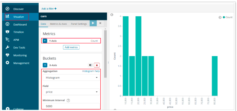
范围分桶与阶梯分桶类似,也是把数字按照阶段进行分组,只不过range方式需要你自己指定每一组的起始和结束大小。