原文链接:http://tecdat.cn/?p=6454
聚类方法用于识别从营销,生物医学和地理空间等领域收集的多变量数据集中的相似对象。它们是不同类型的聚类方法,包括:
- 划分方法
- 分层聚类
- 模糊聚类
- 基于密度的聚类
- 基于模型的聚类
数据准备
- 演示数据集:名为USArrest的内置R数据集
- 删除丢失的数据
- 缩放变量以使它们具有可比性
# Load  and prepare the data

my_data <- USArrests %>%
  na.omit() %>%          # Remove missing values (NA)
  scale()                # Scale variables

# View the firt 3 rows
head(my_data, n = 3)
## Murder Assault UrbanPop Rape
## Alabama 1.2426 0.783 -0.521 -0.00342
## Alaska 0.5079 1.107 -1.212 2.48420
## Arizona 0.0716 1.479 0.999 1.04288距离
get_dist():用于计算数据矩阵的行之间的距离矩阵。与标准dist()功能相比,它支持基于相关的距离测量,包括“皮尔逊”,“肯德尔”和“斯皮尔曼”方法。fviz_dist():用于可视化距离矩阵
res.dist <- get_dist(U
   gradient = list(low = "#00AFBB", mid = "white", high = "#FC4E07"))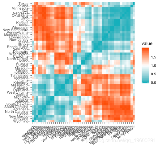
![]()
划分聚类
、算法是将数据集细分为一组k个组的聚类技术,其中k是分析人员预先指定的组的数量。
k-means聚类的替代方案是K-medoids聚类或PAM(Partitioning Around Medoids,Kaufman和Rousseeuw,1990),与k-means相比,它对异常值不太敏感。
以下R代码显示如何确定最佳簇数以及如何在R中计算k-means和PAM聚类。
fviz_nbclust(my_data, kmeans, method = "gap_stat")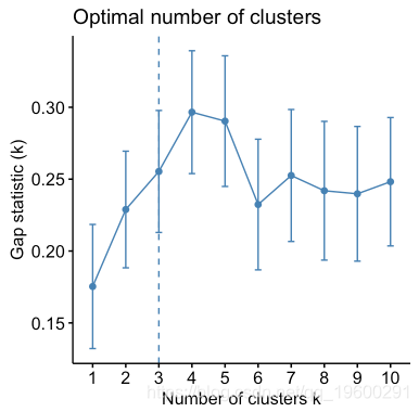
![]()
set.seed(123) # Visualize fviz_cluster(km.res, data = my_data, ellipse.type = "convex", palette = "jco", ggtheme = theme_minimal())

# Compute PAM
pam.res <- pam(my_data, 3)
# Visualize
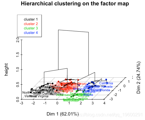
fviz_cluster(pam.res)分层聚类
分层聚类是一种分区聚类的替代方法,用于识别数据集中的组。它不需要预先指定要生成的簇的数量。
# Compute hierarchical clustering res.hc <- USArrests %>% scale() %>% # Scale the data hclust(method = "ward.D2") # Compute hierachical clustering # Visualize using factoextra # Cut in 4 groups and color by groups fviz_dend(res.hc, k = 4, # Cut in four groups color_labels_by_k = TRUE, # color labels by groups rect = TRUE # Add rectangle around groups )

评估聚类倾向
为了评估聚类倾向,可以使用Hopkins的统计量和视觉方法。
- Hopkins统计:如果Hopkins统计量的值接近1(远高于0.5),那么我们可以得出结论,数据集是显着可聚类的。
- 视觉方法:视觉方法通过计算有序相异度图像中沿对角线的方形黑暗(或彩色)块的数量来检测聚类趋势。
R代码:
iris[, -5] %>%    # Remove column 5 (Species)
  scale() %>%     # Scale variables
  get_clust_tendency(n = 50, gradient = gradient.color)
## $hopkins_stat
## [1] 0.8
##
## $plot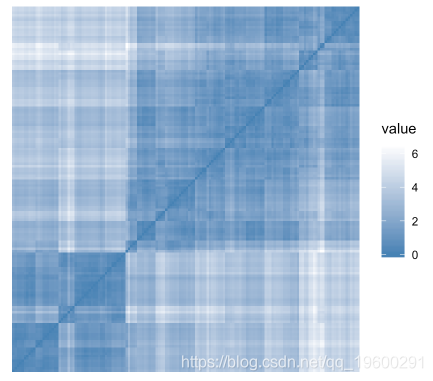
![]()
确定最佳簇数
set.seed(123)

# Compute

res.nbclust <- USArrests %>%
  scale() %>%
   (distance = "euclidean",
          min.nc = 2, max.nc = 10,
          method = "complete", index ="all")
# Visualize
fviz_nbclust(res.nbclust, ggtheme = theme_minimal())## Among all indices:
## ===================
## * 2 proposed 0 as the best number of clusters
## * 1 proposed 1 as the best number of clusters
## * 9 proposed 2 as the best number of clusters
## * 4 proposed 3 as the best number of clusters
## * 6 proposed 4 as the best number of clusters
## * 2 proposed 5 as the best number of clusters
## * 1 proposed 8 as the best number of clusters
## * 1 proposed 10 as the best number of clusters
##
## Conclusion
## =========================
## * According to the majority rule, the best number of clusters is 2 .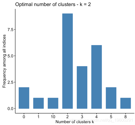
![]()
群集验证统计信息
在下面的R代码中,我们将计算和评估层次聚类方法的结果。
- 计算和可视化层次聚类:
# Enhanced hierarchical clustering, cut in 3 groups res.hc <- iris[, -5] %>% scale() %>% ("hclust", k = 3, graph = FALSE) # Visualize with factoextra (res.hc, palette = "jco", rect = TRUE, show_labels = FALSE)
检查轮廓图:

(res.hc)## cluster size ave.sil.width
## 1 1 49 0.63
## 2 2 30 0.44
## 3 3 71 0.32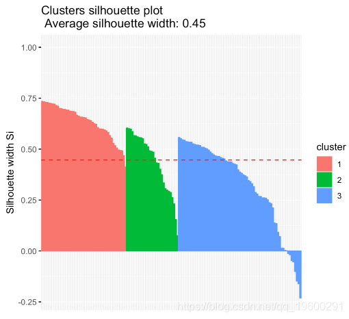
![]()
- 哪些样品有负面轮廓?他们更接近什么集群?
# Silhouette width of observations
sil <- res.hc$silinfo$widths[, 1:3]

# Objects with negative silhouette
neg_sil_index <- which(sil[, 'sil_width'] < 0)
sil[neg_sil_index, , drop = FALSE]
## cluster neighbor sil_width
## 84 3 2 -0.0127
## 122 3 2 -0.0179
## 62 3 2 -0.0476
## 135 3 2 -0.0530
## 73 3 2 -0.1009
## 74 3 2 -0.1476
## 114 3 2 -0.1611
## 72 3 2 -0.2304高级聚类方法
混合聚类方法
- 分层K均值聚类:一种改进k均值结果的混合方法
- HCPC:主成分上的分层聚类
模糊聚类
模糊聚类也称为软聚类方法。标准聚类方法(K-means,PAM),其中每个观察仅属于一个聚类。这称为硬聚类。
基于模型的聚类
在基于模型的聚类中,数据被视为来自两个或多个聚类的混合的分布。它找到了最适合模型的数据并估计了簇的数量。
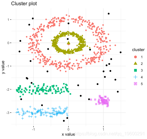
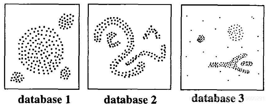
DBSCAN:基于密度的聚类
DBSCAN是Ester等人引入的聚类方法。(1996)。它可以从包含噪声和异常值的数据中找出不同形状和大小的簇(Ester等,1996)。基于密度的聚类方法背后的基本思想源于人类直观的聚类方法。
R链中的DBSCAN的描述和实现
![]()