Written Memories: Understanding, Deriving and Extending the LSTM
When I was first introduced to Long Short-Term Memory networks (LSTMs), it was hard to look past their complexity. I didn’t understand why they were designed they way they were designed, just that they worked. It turns out that LSTMs can be understood, and that, despite their superficial complexity, LSTMs are actually based on a couple incredibly simple, even beautiful, insights into neural networks. This post is what I wish I had when first learning about recurrent neural networks (RNNs).
In this post, we do a few things:
- We’ll define and describe RNNs generally, focusing on the limitations of vanilla RNNs that led to the development of the LSTM.
- We’ll describe the intuitions behind the LSTM architecture, which will enable us to build up to and derive the LSTM. Along the way we will derive the GRU. We’ll also derive a pseudo LSTM, which we’ll see is better in principle and performance to the standard LSTM.
- We’ll then extend these intuitions to show how they lead directly to a few recent and exciting architectures: highway and residual networks, and Neural Turing Machines.
This is a post about theory, not implementations. For how to implement RNNs using Tensorflow, check out my posts Recurrent Neural Networks in Tensorflow I and Recurrent Neural Networks in Tensorflow II.
Contents / quick links:
- Recurrent neural networks
- What RNNs can do; choosing the time step
- The vanilla RNN
- Information morphing and vanishing and exploding sensitivity
- A mathematically sufficient condition for vanishing sensitivity
- A minimum weight initialization for avoid vanishing gradients
- Backpropagation through time and vanishing sensitivity
- Dealing with vanishing and exploding gradients
- Written memories: the intuition behind LSTMs
- Using selectivity to control and coordinate writing
- Gates as a mechanism for selectivity
- Gluing gates together to derive a prototype LSTM
- Three working models: the normalized prototype the GRU and the pseudo LSTM
- Deriving the LSTM
- The LSTM with peepholes
- An empirical comparison of the basic LSTM and the pseudo LSTM
- Extending the LSTM
Prerequisites1
This post assumes the reader is already familiar with:
- Feedforward neural networks
- Backpropagation
- Basic linear algebra
We’ll review everything else, starting with RNNs in general.
Recurrent neural networks
From one moment to the next, our brain operates as a function: it accepts inputs from our senses (external) and our thoughts (internal) and produces outputs in the form of actions (external) and new thoughts (internal). We see a bear and then think “bear”. We can model this behavior with a feedforward neural network: we can teach a feedforward neural network to think “bear” when it is shown an image of a bear.
But our brain is not a one-shot function. It runs repeatedly through time. We see a bear, then think “bear”, then think “run”.2 Importantly, the very same function that transforms the image of a bear into the thought “bear” also transforms the thought “bear” into the thought “run”. It is a recurring function, which we can model with arecurrent neural network (RNN).
An RNN is a composition of identical feedforward neural networks, one for each moment, or step in time, which we will refer to as “RNN cells”. Note that this is a much broader definition of an RNN than that usually given (the “vanilla” RNN is covered later on as a precursor to the LSTM). These cells operate on their own output, allowing them to be composed. They can also operate on external input and produce external output. Here is a diagram of a single RNN cell:

Here is a diagram of three composed RNN cells:

You can think of the recurrent outputs as a “state” that is passed to the next timestep. Thus an RNN cell accepts a prior state and an (optional) current input and produces a current state and an (optional) current output.
Here is the algebraic description of the RNN cell:
where:
- stst and st−1st−1 are our current and prior states,
- otot is our (possibly empty) current output,
- xtxt is our (possibly empty) current input, and
- ff is our recurrent function.
Our brain operates in place: current neural activity takes the place of past neural activity. We can see RNNs as operating in place as well: because RNN cells are identical, they can all be viewed as the same object, with the “state” of the RNN cell being overwritten at each time step. Here is a diagram of this framing:

Most introductions to RNNs start with this “single cell loop” framing, but I think you’ll find the sequential frame more intuitive, particularly when thinking about backpropagation. When starting with the single cell loop framing, RNN’s are said to “unrolled” to obtain the sequential framing above.
What RNNs can do; choosing the time step
The RNN structure described above is incredibly general. In theory, it can do anything: if we give the neural network inside each cell at least one hidden layer, each cell becomes a universal function approximator.3 This means that an RNN cell can emulate any function, from which it follows that an RNN could, in theory, emulate our brain perfectly. Though we know that the brain can theoretically be modeled this way, it’s an entirely different matter to actually design and train an RNN to do this. We are, however, making good progress.
With this analogy of the brain in mind, all we need to do to see how we can use an RNN to handle a task is to ask how a human would handle the same task.
Consider, for example, English-to-French translation. A human reads an English sentence (“the cat sat on the mat”), pauses, and then writes out the French translation (“le chat s’assit sur le tapis”). To emulate this behavior with an RNN, the only choice we have to make (other than designing the RNN cell itself, which for now we treat as a black box) is deciding what the time steps used should be, which determines the form the inputs and outputs, or how the RNN interacts with the external world.
One option is to set the time step according to the content. That is, we might use the entire sentence as a time step, in which case our RNN is just a feed-forward network:
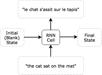
The final state does not matter when translating a single sentence. It might matter, however, if the sentence were part of a paragraph being translated, since it would contain information about the prior sentences. Note that the intial state is indicated above as blank, but when evaluating individual sequences, it can useful to train the initial state as a variable. It may be that the best “a sequence is starting” state representation might not be the blank zero state.
Alternatively, we might say that each word or each character is a time step. Here is an illustration of what an RNN translating “the cat sat” on a per word basis might look like:
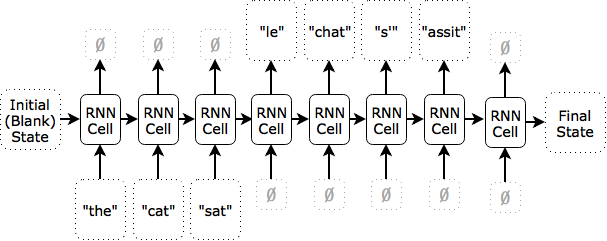
After the first time step, the state contains an internal representation of “the”; after the second, of “the cat”; after the the third, “the cat sat”. The network does not produce any outputs at the first three time steps. It starts producing outputs when it receives a blank input, at which point it knows the input has terminated. When it is done producing outputs, it produces a blank output to signal that it’s finished.
In practice, even powerful RNN architectures like deep LSTMs might not perform well on multiple tasks (here there are two: reading, then translating). To accomodate this, we can split the network into multiple RNNs, each of which specializes in one task. In this example, we would use an “encoder” network that reads in the English (blue) and a separate “decoder” network that reads in the French (orange):
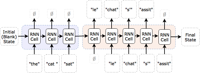
Additionally, as shown in the above diagram, the decoder network is being fed in the last true value (i.e., the target value during training, and the network’s prior choice of translated word during testing). For an example of an RNN encoder-decoder model, see Cho et al. (2014).
Notice that having two separate networks still fits the definition of a single RNN: we can define the recurring function as a split function that takes, alongside its other inputs, an input specifying which split of the function to use.
The time step does not have to be content-based; it can be an actual unit of time. For example, we might consider the time step to be one second, and enforce a reading rate of 5 characters per second. The inputs for the first three time steps would be the c, at sa and t on.
We could also do something more interesting: we can let the RNN decide when its ready to move on to the next input, and even what that input should be. This is similar to how a human might focus on certain words or phrases for an extended period of time to translate them or might double back through the source. To do this, we use the RNN’s output (an external action) to determine its next input dynamically. For example, we might have the RNN output actions like “read the last input again”, “backtrack 5 timesteps of input”, etc. Successful attention-based translation models are a play on this: they accept the entire English sequence at each time step and their RNN cell decides which parts are most relevant to the current French word they are producing.
There is nothing special about this English-to-French translation example. Whatever the human task we choose, we can build different RNN models by choosing different time steps. We can even reframe something like handwritten digit recognition, for which a one-shot function (single time step) is the typical approach, as a many-time step task. Indeed, take a look at some of the MNIST digits yourself and observe how you need to focus on some longer than others. Feedforward neural networks cannot exhibit that behavior; RNNs can.
The vanilla RNN
Now that we’ve covered the big picture, lets take a look inside the RNN cell. The most basic RNN cell is a single layer neural network, the output of which is used as both the RNN cell’s current (external) output and the RNN cell’s current state:

Note how the prior state vector is the same size as the current state vector. As discussed above, this is critical for composition of RNN cells. Here is the algebraic description of the vanilla RNN cell:
where:
- ϕϕ is the activation function (e.g., sigmoid, tanh, ReLU),
- st∈Rnst∈Rn is the current state (and current output),
- st−1∈Rnst−1∈Rn is the prior state,
- xt∈Rmxt∈Rm is the current input,
- W∈Rn×nW∈Rn×n, U∈Rm×nU∈Rm×n, and b∈Rnb∈Rn are the weights and biases, and
- nn and mm are the state and input sizes.
Even this basic RNN cell is quite powerful. Though it does not meet the criteria for universal function approximation within a single cell, it is known that a series of composed vanilla RNN cells is Turing complete and can therefore implement any algorithm. See Siegelmann and Sontag (1992). This is nice, in theory, but there is a problem in practice: training vanilla RNNs with backpropagation algorithm turns out to be quite difficult, even more so than training very deep feedforward neural networks. This difficulty is due to the problems of information morphing and vanishing and exploding sensitivity caused by repeated application of the same nonlinear function.
Information morphing and vanishing and exploding sensitivity4
Instead of the brain, consider modeling the entire world as an RNN: from each moment to the next, the state of the world is modified by a fantastically complex recurring function called time. Now consider how a small change today will affect the world in one hundred years. It could be that something as small as the flutter of a butterfly’s wing will ultimately cause a typhoon halfway around the world.5 But it could also be that our actions today ultimately do not matter. So Einstein wasn’t around to discover relativity? This would have made a difference in the 1950s, but maybe then someone else discovers relativity, so that the difference becomes smaller by the 2000s, and ultimately approaches zero by the year 2050. Finally, it could be that the importance of a small change fluctuates: perhaps Einstein’s discovery was in fact caused by a comment his wife made in response to a butteryfly that happened to flutter by, so that the butterfly exploded into a big change during the 20th century that then quickly vanished.
In the Einstein example, note that the past change is the introduction of new information (the theory of relativity), and more generally that the introduction of this new information was a direct result of our recurring function (the flow of time). Thus, we can consider information itself as a change that is morphed by the recurring function such that its effects vanish, explode or simply fluctuate.
This discussion shows that the state of the world (or an RNN) is constantly changing and that the present can be either extremely sensitive or extremely insensitive to past changes: effects can compound or dissolve. These are problems, and they extend to RNNs (and feedforward neural networks) in general:
-
Information Morphing
First, if information constantly morphs, it is difficult to exploit past information properly when we need it. The best usable state of the information may have occured at some point in the past. On top of learning how to exploit the information today (if it were around in its original, usable form), we must also learn how to decode the original state from the current state, if that is even possible. This leads to difficult learning and poor results.6
It’s very easy to show that information morphing occurs in a vanilla RNN. Indeed, suppose it were possible for an RNN cell to maintain its prior state completely in the absence of external inputs. Then F(x)=ϕ(Wst−1+b)F(x)=ϕ(Wst−1+b) is the identity function with respect to st−1st−1. But the identity function is linear and F(x)F(x) is nonlinear, so we have a contradiction. Therefore, an RNN cell inevitably morphs the state from one time step to the next. Even the trivial task of outputting st=xtst=xt is impossible for a vanilla RNN.
This is the root cause of what is known in some circles as the degradation problem. See, e.g., He et al. (2015). The authors of He et al. claims this is “unexpected” and “counterintuitive”, but I hope this discussion shows that the degradation problem, or information morphing, is actually quite natural (and in many cases desirable). We’ll see below that although information morphing was not among the original motivations for introducing LSTMs, the principle behind LSTMs happens to solve the problem effectively. In fact, the effectiveness of the residual networks used by He at al. (2015) is a result of the fundamental principle of LSTMs.
-
Vanishing and Exploding Gradients
Second, we train RNNs using the backpropagation algorithm. But backpropagation is a gradient-based algorithm, and vanishing and exploding “sensitivity” is just another way of saying vanishing and exploding gradients (the latter is the accepted term, but I find the former more descriptive). If the gradients explode, we can’t train our model. If they vanish, it’s difficult for us to learn long-term dependencies, since backpropagation will be too sensitive to recent distractions. This makes training difficult.
I’ll come back to the difficulty of training RNNs via backpropagation in a second, but first I’d like to give a short mathematical demonstration of how easy it is for the vanilla RNN to suffer from the vanishing gradients and what we can do to help avoid this at the start off training.
A mathematically sufficient condition for vanishing sensitivity
In this section I give a mathematical proof of a sufficient condition for vanishing sensitivity in vanilla RNNs. It is essentially the same as the proof of the similar result in Pascanu et al. (2013), but I think you will find this presentation easier to follow. The proof here also takes advantage of the mean value theorem to go one step further than Pascanu et al. and reach a slightly stronger result, effectively showing vanishing causation rather than vanishing sensitivity.7 Note that mathematical analyses of vanishing and exploding gradients date back to the early 1990s, in Bengio et al. (1994) and Hochreiter (1991) (original in German, relevant portions summarized in Hochreiter and Schmidhuber (1997)).
Let stst be our state vector at time tt and let ΔvΔv be the change in a vector vv induced by a change in the state vector, ΔstΔst, at time tt. Our objective is to provide a mathematically sufficient condition so that the change in state at time step t+kt+k caused by a change in state at time step tt vanishes as n→∞n→∞; i.e., we will prove a sufficient condition for:
By constrast, Pascanu et al. (2013) proved the same sufficient condition for the following result, which can easily be extended to obtain the above:
To begin, from our definition of a vanilla RNN cell, we have:
Applying the mean value theorem in several variables, we get that there exists c∈[zt, zt+Δzt]c∈[zt, zt+Δzt] such that:
Now let ∥A∥∥A∥ represent the matrix 2-norm, ∣v∣∣v∣ the Euclidean vector norm, and define:
Note that for the logistic sigmoid, γ≤14γ≤14, and for tanh, γ≤1γ≤1.
Taking the vector norm of each side, we obtain, where the first inequality comes from the definition of the 2-norm (applied twice), and second from the definition of supremum:
By expanding this formula over kk time steps we get ∣Δst+k∣≤∥γW∥k∣Δst∣∣Δst+k∣≤∥γW∥k∣Δst∣ so that:
Therefore, if ∥γW∥<1∥γW∥<1, we have that ∣Δst+k∣∣Δst∣∣Δst+k∣∣Δst∣ decreases exponentially in time, and have proven a sufficient condition for:
When will ∥γW∥<1∥γW∥<1? γγ is bounded to 1414 for the logistic sigmoid and to 1 for tanh, which tells us that the sufficient condition for vanishing gradients is for ∥W∥∥W∥ to be less than 4 or 1, respectively.
An immediate lesson from this is that if our weight initializations for WW are too small, our RNN may be unable to learn anything right off the bat, due to vanishing gradients. Let’s now extend this analysis to determine a desirable weight initialization.
A minimum weight initialization for avoid vanishing gradients
It is beneficial to find a weight initialization that will not immediately suffer from this problem. Extending the above analysis to find the initialization of WW that gets us as close to equality as possible leads to a nice result.
First, let us assume that ϕ=tanhϕ=tanh and take γ=1γ=1,8 but you could just as easily assume that ϕ=σϕ=σ and take γ=14γ=14 to reach a different result.
Our goal is to find an initialization of W for which:
- ∥γW∥=1∥γW∥=1.
- We get as close to equality as possible in equation (1).
From point 1, since we took γγ to be 1, we have ∥W∥=1∥W∥=1. From point 2, we get that we should try to set all singular values of WW to 1, not just the largest. Then, if all singular values of WW equal 1, that means that the norm of each column of WW is 1 (since each column is WeiWei for some elementary basis vector eiei and we have ∣Wei∣=∣ei∣=1∣Wei∣=∣ei∣=1). That means that for column jj we have:
There are nn entries in column jj, and we are choosing each from the same random distribution, so let us find a distribution for a random weight ww for which:
Now let’s suppose we want to initialize ww uniformly in the interval [−R, R][−R, R]. Then the mean of ww is 0, so that, by definition, E(w2)E(w2) is its variance, V(w)V(w). The variance of a uniform distribution over the interval [a, b][a, b] is given by (b−a)212(b−a)212, from which we get V(w)=R23V(w)=R23. Substituting this into our equation we get:
So that:
This suggests that we initialize our weights from the uniform distribution over the interval:
This is a nice result because it is the Xavier-Glorot initialization for a square weight matrix, yet was motivated by a different idea. The Xavier-Glorot initialization, introduced by Glorot and Bengio (2010), has proven to be an effective weight initialization prescription in practice. More generally, the Xavier-Glorot prescription applies to mm-by-nn weight matrices used in a layer that has an activation function whose derivative is near one at the origin (like tanhtanh), and says that we should initialize our weights according to a uniform distribution of the interval:
You can easily modify the above analysis to obtain initialization prescriptions when using the logistic sigmoid (use γ=14γ=14) and when initializing the weights according to a different random distribution (e.g., a Gaussian distribution).
Backpropagation through time and vanishing sensitivity
Training an RNN with backpropagation is very similar to training a feedforward network with backpropagation. Since it is assumed you are already familiar with backpropagation generally, there are only a few comments to make:
-
We backpropagate errors through time
For RNNs we need to backpropagate errors from the current RNN cell back through the state, back through time, to prior RNN cells. This allows the RNN to learn to capture long term time dependencies. Because the model’s parameters are shared across RNN cells (each RNN cell has identical weights and biases), we need to calculate the gradient with respect to each time step separately and then add them up. This is similar to the way we backpropagate errors to shared parameters in other models, such as convolutional networks.
-
There is a trade-off between weight update frequency and accurate gradients
For all gradient-based training algorithms, there is an unavoidable trade-off between (1) frequency of parameter updates (backward passes), and (2) accurate long-term gradients. To see this, consider what happens when we update the gradients at each step, but backpropagate errors more than one step back:
- At time tt we use our current weights, WtWt, to calculate the current output and current state, otot and stst.
- Second, we use otot to run a backward pass and update WtWt to Wt+1Wt+1.
- Third, at time t+1t+1, we use Wt+1Wt+1 and stst, as calculated in step 1 using the original WtWt, to calculate ot+1ot+1 and st+1st+1.
- Finally, we use ot+1ot+1 to run a backward pass. But ot+1ot+1 was computed using WtWt, which means the gradients we compute for weights at time step tt are evaluated at our old weights, WtWt, and not the current weights, Wt+1Wt+1. They are thus only an estimate of the gradient, if it were computed with respect to the current weights. This effect will only compound as we backpropagate errors even further.
We could compute more accurate gradients by doing fewer parameter updates (backward passes), but then we might be giving up training speed (which can be particularly harmful at the start of training). Note the similarity to the trade off to the one faces by choosing a mini-batch size for mini-batch gradient descent: the larger the batch size, the more accurate the estimate of the gradient, but also the fewer gradient updates.
We could also choose to not propagate errors back more steps than the frequency of our parameter updates, but then we are not calculating the full gradient of the cost with respect to the weights and this is just the flip-side of the coin; the same trade-off occurs.
This effect is discussed in Williams and Zipser (1995), which provides an excellent overview of the options for calculating gradients for gradient-based training algorithms.
-
Vanishing gradients plus shared parameters means unbalanced gradient flow and oversensitivity to recent distractions
Consider a feedforward neural network. Exponentially vanishing gradients mean that changes made to the weights in the earlier layers will be exponentially smaller than those made to the weights in later layers. This is bad, even if we train the network for exponentially longer, so that the early layers eventually learn. To see this, consider that during training the early layers and later layers learn how to communicate with each other. The early layers initially send crude signals, so the later layers quickly become very good at interpretting these crude signals. But then the early laters are encouraged to learn how to produce better crude symbols rather than producing more sophisticated ones.
RNNs have it worse, because unlike for feedforward nets, the weights in early layers and later layers are shared. This means that instead of simply miscommunicating, they can directly conflict: the gradient to a particular weight might be positive in the early layers but negative in the later layers, resulting in a negative overall gradient, so that the early layers are unlearning faster than they can learn. In the words of Hochreiter and Schmidhuber (1997): “Backpropagation through time is too sensitive to recent distractions.”
-
Therefore it makes sense to truncate backpropagation
Limiting the number of steps that we backpropagate errors in training is called truncating the backpropagation. Notice immediately that if the input/output sequence we are fitting is infinitely long we must truncate the backpropagation, else our algorithm would halt on the backward pass. If the sequence is finite but very long, we may still need to truncate the backpropagation due to computation infeasability.
However, even if we had a supercomputer that could instantly backpropagate an error an infinite number of timesteps, point 2 above tells us that we need to truncate our backpropagation due to our gradients becoming inaccurate as a result of weight updates.
Finally, vanishing gradients create yet another reason for us truncate our backpropagation. If our gradients vanish, then gradients that are backpropagated many steps will be very small and have a negligible effect on training.
Note that we choose not only how often to truncate backpropagation, but also how often to update our model parameters. See my post on Styles of Truncated Backpropagation for an empirical comparison of two possible methods of truncation, or refer to the discussion in Williams and Zipser (1995).
-
There is also such thing as forward propagation of gradient components
Something useful to know (in case you come up with the idea yourself), is that backpropagation is not our only choice for training RNNs. Instead of backpropagating errors, we can also propagate gradient components forward, allowing us to compute the error gradient with respect to the weights at each time step. This alternate algorithm is called “real-time recurrent learning (RTRL)”. Full RTRL is too computationally expensive to be practical, running in O(n4)O(n4) time (as compared to truncated backpropagation, which is O(n2)O(n2) when parameters are updated with the same frequency as backward passes). Similar to how truncated backpropagation approximates full backpropagation (whose time complexity, O(n2L)O(n2L), can be much higher than RTRL when the number of time steps, LL, is large), there exists an approximate version of RTRL called subgrouped RTRL. It promises the same time complexity as truncated backpropagation (O(n2)O(n2)) when the size of the subgroups is fixed, but is qualitatively different in how it approximates the gradient. Note that RTRL is a gradient-based algorithm and therefore suffers from the vanishing and exploding gradient problem. You can learn more about RTRL in Williams and Zipser (1995). RTRL is just something I wanted to bring to your attention, and beyond our scope; in this post, I assume the use of truncated backpropagation to calculate our gradients.
Dealing with vanishing and exploding gradients
If our gradient explodes backpropagation will not work because we will get NaN values for the gradient at early layers. An easy solution for this is to clip the gradient to a maximum value, as proposed by Mikolov (2012) and reasserted in Pascanu et al. (2013). This works in practice to prevent NaN values and allows training to continue.
Vanishing gradients are tricker to deal with in vanilla RNNs. We saw above that good weight initializations are crucial, but this only impacts the start of training – what about the middle of training? The approach suggested in Pascanu et al. (2013) is to introduce a regularization term that enforces constant backwards error flow. This is an easy solution that seems to work for the few experiments on which it was tested in Pascanu et al. (2013). Unfortunately, it is difficult to find a justification for why this should work all the time, because we are imposing an opinion about the way gradients should flow on the model. This opinion may be correct for some tasks, in which case our imposition will help achieve better results. However, it may be that for some tasks we want gradients to vanish completely, and for others, it may be that we want them to grow. In these cases, the regularizer would detract from the model’s performance, and there doesn’t seem to be any justification for saying that one situation is more common than the other. LSTMs avoid this issue altogether.
Written memories: the intuition behind LSTMs
Very much like the messages passed by children playing a game of broken telephone, information is morphed by RNN cells and the original message is lost. A small change in the original message may not have made any difference in the final message, or it may have resulted in something completely different.
How can we protect the integrity of messages? This is the fundamental principle of LSTMs: to ensure the integrity of our messages in the real world, we write them down. Writing is a delta to the current state: it is an act of creation (pen on paper) or destruction (carving in stone); the subject itself does not morph when you write on it and the error gradient on the backward-pass is constant.
This is precisely what was proposed by the landmark paper of Hocreiter and Schmidhuber (1997), which introduced the LSTM. They asked: “how can we achieve constant error flow through a single unit with a single connection to itself [i.e., a single piece of isolated information]?”
The answer, quite simply, is to avoid information morphing: changes to the state of an LSTM are explicitly written in, by an explicit addition or subtraction, so that each element of the state stays constant without outside interference: “the unit’s activation has to remain constant … this will be ensured by using the identity function”.
The fundamental principle of LSTMs: Write it down.
To ensure the integrity of our messages in the real world, we write them down. Writing is an incremental change that can be additive (pen on paper) or subtractive (carving in rock), and which remains unchanged absent outside interference. In LSTMs, everything is written down and, assuming no interference from other state units or external inputs, carries its prior state forward.
Practically speaking, this means that any state changes are incremental, so that st+1=st+Δst+1st+1=st+Δst+1.9
Now Hochreiter and Schmidhuber observed that just “writing it down” had been tried before, but hadn’t worked so well. To see why, consider what happens when we keep writing in changes:
Some of our writes are positive, and some are negative, so it’s not true that our canvas necessarily blows up: our writes could theoretically cancel each other out. However, it turns out that it’s quite hard to learn how to coordinate this. In particular, at the start of training, we start with random initializations and our network is making some fairly random writes. From the very start of training, we end up with something that looks like this:

Even if we eventually learn to coordinate our writes properly, it’s very difficult to record anything useful on top of that chaos (albeit, in this example, very pretty and somewhat regular chaos that was worth $140 millionabout 10 years ago). This is the fundamental challenge of LSTMs: Uncontrolled and uncoordinated writing causes chaos and overflow from which it can be very hard to recover.
The fundamental challenge of LSTMs: Uncontrolled and uncoordinated writing.
Uncontrolled and uncoordinated writes, particularly at the start of training when writes are completely random, create a chaotic state that leads to bad results and from which it can be difficult to recover.
Hochreiter and Schmidhuber recognized this problem, splitting it into several subproblems, which they termed “input weight conflict”, “output weight conflict”, the “abuse problem”, and “internal state drift”. The LSTM architecture was carefully designed in order to overcome these problems, starting with the idea of selectivity.
Using selectivity to control and coordinate writing
According to the early literature on LSTMs, the key to overcoming the fundamental challenge of LSTMs and keeping our state under control is to be selective in three things: what we write, what we read (because we need to read something to know what to write), and what we forget (because obselete information is a distraction and should be forgotten).
Part of the reason our state can become so chaotic is that the base RNN writes to every element of the state. This is a problem I suffer from a lot. I have a paper in front of my computer and I write down a lot of things on the same paper. When it fills I take out the paper under it and start writing on that one. The cycle repeats and I end up with a bunch of papers on my desk that contain an overwhelming amount of gibberish.
Hochreiter and Schmidhuber describe this as “input weight conflict”: if each unit is being written to by all units at each time step, it will collect a lot of useless information, rendering its original state unusable. Thus, the RNN must learn how to use some of its units to cancel out other incoming writes and “protect” the state, which results in difficult learning.
First form of selectivity: Write selectively.
To get the most out of our writings in the real world, we need to be selective about what we write; when taking class notes, we only record the most important points and we certainly don’t write our new notes on top of our old notes. In order for our RNN cells to do this, they need a mechanism for selective writing.
The second reason our state can become chaotic is the flip side of the first: for each write it makes, the base RNN reads from every element of the state. As a mild example: if I’m writing a blog post on the intuition behind LSTMs while on vacation in a national park with a wild bear on the loose, I might include the things I’ve been reading about bear safety in my blog post. This is just one thing, and only mildly chaotic, but imagine what this post would look like if I included all the things…
Hochreiter and Schmidhuber describe this as “output weight conflict”: if irrelevant units are read by all other units at each time step, they produce a potentially huge influx of irrelevant information. Thus, the RNN must learn how to use some of its units to cancel out the irrelevant information, which results in difficult learning.
Note the difference between reads and writes: If we choose not to read from a unit, it cannot affect any element of our state and our read decision impacts the entire state. If we choose not to write to a unit, that impacts only that single element of our state. This does not mean the impact of selective reads is more significant than the impact of selective writes: reads are summed together and squashed by a non-linearity, whereas writes are absolute, so that the impact of a read decision is broad but shallow, and the impact of a write decision is narrow but deep.
Second form of selectivity: Read selectively.
In order to perform well in the real-world, we need to apply the most relevant knowledge by being selective in what we read or consume. In order for our RNN cells to do this, they need a mechanism for selective reading.
The third form of selectivity relates to how we dispose of information that is no longer needed. My old paper notes get thrown out. Otherwise I end up with an overwhelming number of papers, even if I were to be selective in writing them. Unused files in my Dropbox get overwritten, else I would run out of space, even if I were to be selective in creating them.
This intuition was not introduced in the original LSTM paper, which led the original LSTM model to have trouble with simple tasks involving long sequences. Rather, it was introduced by Gers et al. (2000). According to Gers et al., in some cases the state of the original LSTM model would grow indefinitely, eventually causing the network to break down. In other words, the original LSTM suffered from information overload.
Third form of selectivity: Forget selectively.
In the real-world, we can only keep so many things in mind at once; in order to make room for new information, we need to selectively forget the least relevant old information. In order for our RNN cells to do this, they need a mechanism for selective forgetting.
With that, there are just two more steps to deriving the LSTM:
- we need to determine a mechanism for selectivity, and
- we need to glue the pieces together.
Gates as a mechanism for selectivity
Selective reading, writing and forgetting involves separate read, write and forget decisions for each element of the state. We will make these decisions by taking advantage of state-sized read, write and forget vectors with values between 0 and 1 specifying the percentage of reading, writing and forgetting that we do for each state element. Note that while it may be more natural to think of reading, writing and forgetting as binary decisions, we need our decisions to be implemented via a differentiable function. The logistic sigmoid is a natural choice since it is differentiable and produces continuous values between 0 and 1.
We call these read, write and forget vectors “gates”, and we can compute them using the simplest function we have, as we did for the vanilla RNN: the single-layer neural network. Our three gates at time step tt are denoted itit, the input gate (for writing), otot, the output gate (for reading) and ftft, the forget gate (for remembering). From the names, we immediately notice that two things are backwards for LSTMs:
- Admittedly this is a bit of a chicken and egg, but I would usually think of first reading then writing. Indeed, this ordering is strongly suggested by the RNN cell specification–we need to read the prior state before we can write to a new one, so that even if we are starting with a blank initial state, we are reading from it. The names input gate and output gate suggest the opposite temporal relationship, which the LSTM adopts. We’ll see that this complicates the architecture.
- The forget gate is used for forgetting, but it actually operates as a remember gate. E.g., a 1 in a forget gate vector means remember everything, not forget everything. This makes no practical difference, but might be confusing.
Here are the mathematical definitions of the gates (notice the similarities):
We could use more complicated functions for the gates as well. A simple yet effective recent example is the use of “multiplicative integration”. See Wu et al. (2016).
Let’s now take a closer look at how our gates interact.
Gluing gates together to derive a prototype LSTM
If there were no write gate, read selectivity says that we should use the read gate when reading the prior state in order to produce the next write to the state (as discussed above, the read naturally comes before the write when we are zoomed in on a single RNN cell). The fundamental principle of LSTMs says that our write will be incremental to the prior state; therefore, we are calculating ΔstΔst, not stst. Let’s call this would-be ΔstΔst ourcandidate write, and denote it s~ts~t.
We calculate s~ts~t the same way we would calculate the state in a vanilla RNN, except that instead of using the prior state, st−1st−1, we first multiply the prior state element-wise by the read gate to get the gated prior state, ot⊙st−1ot⊙st−1:
Note that ⊙⊙ denotes element-wise multiplication, and otot is our read gate (output gate).
s~ts~t is only a candidate write because we are applying selective writing and have a write gate. Thus, we multiply s~ts~t element-wise by our write gate, itit, to obtain our true write, it⊙s~tit⊙s~t.
The final step is to add this to our prior state, but forget selectivity says that we need to have a mechanism for forgetting. So before we add anything to our prior state, we multiply it (element-wise) by the forget gate (which actually operates as a remember gate). Our final prototype LSTM equation is:
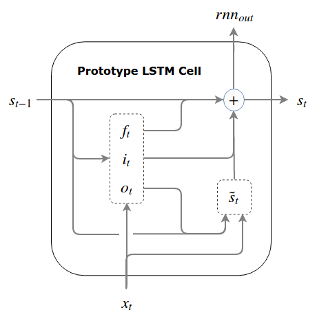
If we gather all of our equations together, we get the full spec for our prototype LSTM cell (note that stst is also the cell’s external output at each time step):
The Prototype LSTM
At the risk of distracting you from the equations (which are far more descriptive), here is what the data flow looks like:
In theory, this prototype should work, and it would be quite beautiful if it did. In practice, the selectivity measures taken are not (usually) enough to overcome the fundamental challenge of LSTMs: the selective forgets and the selective writes are not coordinated at the start of training which can cause the state to quickly become large and chaotic. Further, since the state is potentially unbounded, the gates and the candidate write will often become saturated, which causes problems for training.
This was observed by Hochreiter and Schmidhuber (1997), who termed the problem “internal state drift”, because “if the [writes] are mostly positive or mostly negative, then the internal state will tend to drift away over time”. It turns out that this problem is so severe that the prototype we created above tends to fail in practice, even with very small initial learning rates and carefully chosen bias initializations. The clearest empirical demonstration of this can be found in Greff et al. (2015), which contains an empirical comparison of 8 LSTM variants. The worst performing variant, often failing to converge, is substantially similar to the prototype above.
By enforcing a bound on the state to prevent it from blowing up, we can overcome this problem. There are a few ways to do this, which lead to different models of the LSTM.
Three working models: the normalized prototype, the GRU and the pseudo LSTM
The selectivity measures taken in our prototype LSTM were not powerful enough to overcome the fundamental challenge of LSTMs. In particular, the state, which is used to compute both the gates and the candidate write can grow unbounded.
I’ll cover three options, each of which bounds the state in order to give us a working LSTM:
The normalized prototype: a soft bound via normalization
We can impose a soft bound by normalizing the state. One method that has worked for me in preliminary tests is simply dividing stst by Var(st)+1−−−−−−−−−√Var(st)+1, where we add 1 to prevent the initially zero state from blowing up. We might also subtract the mean state before dividing out the variance, but this did not seem to help in preliminary tests. We might then consider adding in scale and shift factors for expressiveness, a la layer normalization10, but then the model ventures into layer normalized LSTM territory (and we may want to compare it to other layer normalized LSTM models).
In any case, this provides a method for creating a soft bound on the state, and has performed slightly better for me in preliminary tests than regular LSTMs (including the pseudo LSTM derived below).
The GRU: a hard bound via write-forget coupling, or overwriting
One way to impose a hard bound on the state and coordinate our writes and forgets is to explicitly link them; in other words, instead of doing selective writes and selective forgets, we forego some expressiveness and do selective overwrites by setting our forget gate equal to 1 minus our write gate, so that:
This works because it turns stst into an element-wise weighted average of st−1st−1 and s~ts~t, which is bounded if both st−1st−1 and s~ts~t are bounded. This is the case if we use ϕ=tanhϕ=tanh (whose output is bound to (-1, 1)).
We’ve now derived the gated recurrent unit (GRU). To conform for the GRU terminology used in the literature, we call the overwrite gate an update gate and label it ztzt. Note that although called an “update” gate, it operates as “do-not-update” gate by specifying the percentage of the prior state that we don’t want to overwrite. Thus, the update gate, ztzt, is the same as the forget gate from our prototype LSTM, ftft, and the write gate is calculated by 1−zt1−zt.
Note that, for whatever reason, the authors who introduced the GRU called their read gate a reset gate (at least we get to use rtrt for it!).
The GRU
At the risk of distracting you from the equations (which are far more descriptive), here is what the data flow looks like:
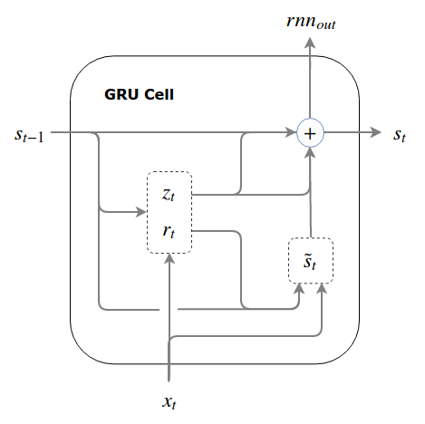
This is the GRU cell first introduced by Cho et al. (2014). I hope you agree that the derivation of the GRU in this post was motivated at every step. There hasn’t been a single arbitrary “hiccup” in our logic, as there will be in order for us to arrive at the LSTM. Contrary to what some authors have written (e.g., “The GRU is an alternative to the LSTM which is similarly difficult to justify” - Jozefowicz et al. (2015)), we see that the GRU is a very natural architecture.
The Pseudo LSTM: a hard bound via non-linear squashing
We now take the second-to-last step on our journey to full LSTMs, by using a third method to bind our state: we pass the state through a squashing function (e.g., the logistic sigmoid or tanh). The hiccup here is that we cannot apply the squashing function to the state itself (for this would result in information morphing and violate our fundamental principle of LSTMs). Instead, we pass the state through the squashing function every time we need to use it for anything except making incremental writes to it. By doing this, our gates and candidate write don’t become saturated and we maintain good gradient flow.
To this point, our external output has been the same as our state, but here, the only time we don’t squash the state is when we make incremental writes to it. Thus, our cell’s output and state are different.
This is an easy enough modification to our prototype. Denoting our new squashing function by ϕϕ (it does not have to be the same as the nonlinearity we use to compute the candidate write but tanh is generally used for both in practice):
The Pseudo LSTM
At the risk of distracting you from the equations (which are far more descriptive), here is what the data flow looks like:
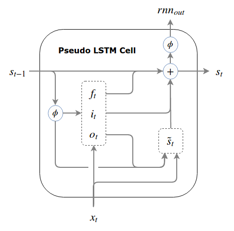
The pseudo LSTM is almost an LSTM - it’s just backwards. From this presentation, we see clearly that the only motivated difference between the GRU and the LSTM is the approach they take to bounding the state. We’ll see that this pseudo LSTM has some advantages over the standard LSTM.
Deriving the LSTM
There are a number of LSTM variants used in the literature, but the differences between them are not so important for our purposes. They all share one key difference with our pseudo LSTM: the real LSTM places the read operation after the write operation.
LSTM Diff 1 (the LSTM hiccup): Read comes after write. This forces the LSTM to pass a shadow state between time steps.
If you read Hochreiter and Schmidhuber (1997) you will observe that they were thinking of the state (as we’ve been using state so far) as being separate from the rest of the RNN cell.11 Hochreiter and Schmidhuber thought of the state as a “memory cell” that had a “constant error” (because absent reading and writing, it carries the state forward and has a constant gradient during backpropagation). Perhaps this is why, viewing the state as a separate memory cell, they saw the order of operations as inputs (writes) followed by outputs (reads). Indeed, most diagrams of the LSTM, including the ones in Hochreiter and Schmidhuber (1997) and Graves (2013) are confusing because they focus on this “memory cell” rather than on the LSTM cell as a whole.12 I don’t include examples here so as to not distract from raw understanding.
This difference in read-write order has the following important implication: We need to read the state in order to create a candidate write. But if creating the candidate write comes before the read operation inside our RNN cell, we can’t do that unless we pass a pre-gated “shadow state” from one time step to the next along with our normal state. The write-then-read order thus forces the LSTM to pass a shadow state from RNN cell to RNN cell.
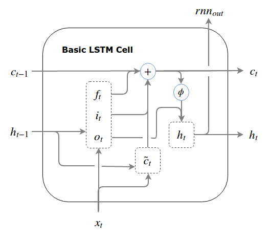
Going forward, to conform to the common letters used in describing the LSTM, we rename the main state, stst, toctct (c is for cell, or constant error). We’ll make the corresponding change to our candidate write, which will now be c~tc~t. We will also introduce a separate shadow state, htht (h is for hidden state) that will has the same size as our regular state. ht−1ht−1 is analogous to the gated prior state from our prototype LSTM, ot⊙st−1ot⊙st−1, except that it is squashed by a non-linearity (to impose a bound on the values used to compute the candidate write). Thus the prior state our LSTM receives at time step tt is a tuple of closely-related vectors: (ct−1, ht−1)(ct−1, ht−1), where ht−1=ot−1⊙ϕ(ct−1)ht−1=ot−1⊙ϕ(ct−1).
This is truly a hiccup, and not because it makes things more complicated (which it does). It’s a hiccup because we end up using a read gate calculated at time t−1t−1, using the shadow state from time t−2t−2 and the the inputs from time t−1t−1, in order to gate the relevant state information for use at time tt. This is like day trading based on yesterday’s news.
Our hiccup created an ht−1ht−1, the presence of which goes on to create two more differences to our pseudo LSTM:
First, instead of using the (squashed) ungated prior state, ϕ(ct−1)ϕ(ct−1), to compute the gates, the standard LSTM uses ht−1=ot−1⊙ϕ(ct−1)ht−1=ot−1⊙ϕ(ct−1), which has been subjected to a read gate, and an outdated read gate at that.
LSTM Diff 2: Gates are computed using the gated shadow state, ht−1=ot−1⊙ϕ(ct−1)ht−1=ot−1⊙ϕ(ct−1), instead of a squashed main state, ϕ(ct−1)ϕ(ct−1).
Second, instead of using the (squashed) ungated state, ϕ(ct)ϕ(ct) as the LSTM’s external output, the standard LSTM uses ht=ot⊙ϕ(ct)ht=ot⊙ϕ(ct), which has been subjected to a read gate.
LSTM Diff 3: The LSTM’s external output is the gated shadow state, ht=ot⊙ϕ(ct)ht=ot⊙ϕ(ct), instead of a squashed main state, ϕ(ct)ϕ(ct).
While we can see how these differences came to be, as a result of the “memory cell” view of the LSTM’s true state, at least the first and third lack a principled motivation (the second can be interpreted as asserting that information that is irrelevant for the candidate write is also irrelevant for gate computations, which makes sense). Thus, while I strongly disagreed above with Jozefowicz et al. (2015) about the GRU being “difficult to justify”, I agree with them that there are LSTM components whose “purpose is not immediately apparent”.
We will now rewrite our pseudo LSTM backwards, taking into account all three differences, to get a real LSTM. It now receives two quantities as the prior state, ct−1ct−1 and ht−1ht−1, and produces two quantities which it will pass to the next time step, ctct and htht. The LSTM we get is quite “normal”: this is the version of the LSTM you will find implemented as the “BasicLSTMCell” in Tensorflow.
The basic LSTM
At the risk of distracting you from the equations (which are far more descriptive), here is what the data flow looks like:
The LSTM with peepholes
The potential downside of LSTM Diff 2 (hiding of potentially relevant information) was recognized by Gers and Schmidhuber (2000), who introduced “peephole” connections in response. Peepholes connections include the original unmodified prior state, ct−1ct−1 in the calculation of the gates. In introducing these peepholes, Gers and Schmidhuber (2000) also noticed the outdated input to the read gate (due to LSTM Diff 1), and partially fixed it by moving the calculation of the read gate, otot, to come after the calculation of ctct, so that otot uses ctct instead of ct−1ct−1 in its peephole connection.
Making these changes, we get one of the most common variants of the LSTM. This is the architecture used inGraves (2013). Note that each PxPx is an n×nn×n matrix (a peephole matrix), much like each WxWx.
The LSTM with peepholes
An empirical comparison of the basic LSTM and the pseudo LSTM
I now compare the basic LSTM to our pseudo LSTM to see if LSTM Diffs 1, 2 and 3 really are harmful. All combinations of the three differences are tested, for a total of 8 possible architectures:
-
Pseudo LSTM: as above.
-
Pseudo LSTM plus LSTM Diff 1: Shadow state containing read-gated squashed state, ot−1⊙ϕ(ct−1)ot−1⊙ϕ(ct−1), is passed to time step tt, where it used in computation of the candidate write only. Gates and outputs are calculated using the ungated squashed state.
-
Pseudo LSTM plus LSTM Diffs 1 and 2: Shadow state containing read-gated squashed state, ot−1⊙ϕ(ct−1)ot−1⊙ϕ(ct−1), is passed to time step tt, where it used in computation of the candidate write and each of the three gates.
-
Pseudo LSTM plus LSTM Diffs 1 and 3: Shadow state containing read-gated squashed state, ot−1⊙ϕ(ct−1)ot−1⊙ϕ(ct−1), is passed to time step tt, where it used in computation of the candidate write only. The shadow state, ot⊙ϕ(ct)ot⊙ϕ(ct), is also used as the cell output at time step tt (i.e., the cell output is read-gated).
-
Pseudo LSTM plus LSTM Diff 2: Read-gated squashed prior state, ot⊙ϕ(st−1)ot⊙ϕ(st−1), is used in place of squashed prior state, ϕ(st−1)ϕ(st−1), to compute the write gate and forget gate.
-
Pseudo LSTM plus LSTM Diffs 2 and 3: Read-gated squashed prior state, ot⊙ϕ(st−1)ot⊙ϕ(st−1), is used in place of squashed prior state, ϕ(st−1)ϕ(st−1), to compute the write gate and forget gate, and also to gate the cell output.
-
Pseudo LSTM plus LSTM Diff 3: Pseudo LSTM using read-gated squashed state as its external output, ot⊙ϕ(st)ot⊙ϕ(st), instead of squashed state, ϕ(st)ϕ(st).
-
Basic LSTM: as above.
In architectures 5-7, the read gate is calculated at time tt (i.e., they do not incorporate the time delay caused by LSTM Diff 1). All architectures use a forget gate bias of 1, and read/write gate biases of 0.
Using the PTB dataset, I run 5 trials of up to 20 epochs of each. Training is cut short if the loss does not fall after 2 epochs, and the minimum epoch validation loss is reported. Gradients are calculated with respect to a softmax/cross-entropy loss via backpropagation truncated to 30 steps, and learning is performed in batches of 30 with an AdamOptimizer and learning rates of 3e-3, 1e-3, 3e-4, and 1e-4. The state size used is 250. No dropout, layer normalization or other features are added. Architectures are composed of a single layer of RNN cells (i.e., this is not a comparison of deep architectures). RNN inputs are passed through an embedding layer, and RNN outputs are passed through a softmax.
The best epoch validation losses, shown as the average of 5 runs with a 95% confidence interval, are as follows (lower is better):
| LR | 1 (pseudo) | 2 {1} | 3 {1,2} | 4 {1,3} | 5 {2} | 6 {2,3} | 7 {3} | 8 (basic) |
|---|---|---|---|---|---|---|---|---|
| 3e-03 | 433.7 ± 10.6 | 430.6 ± 6.1 | 390.3 ± 1.2 | 424.5 ± 3.5 | 389.0 ± 1.4 | 399.1 ± 2.4 | 425.7 ± 1.4 | 396.2 ± 1.6 |
| 1e-03 | 387.2 ± 0.8 | 388.6 ± 1.0 | 388.7 ± 0.6 | 414.3 ± 2.5 | 386.0 ± 0.8 | 396.3 ± 1.9 | 413.9 ± 2.4 | 396.6 ± 0.9 |
| 3e-04 | 389.2 ± 0.6 | 391.1 ± 0.8 | 391.3 ± 0.8 | 407.9 ± 4.3 | 388.8 ± 0.6 | 397.7 ± 1.5 | 408.7 ± 1.7 | 398.8 ± 2.1 |
| 1e-04 | 403.9 ± 1.0 | 403.9 ± 0.8 | 404.2 ± 1.3 | 419.7 ± 0.4 | 403.1 ± 1.2 | 416.8 ± 1.4 | 419.9 ± 1.4 | 418.1 ± 1.2 |
We see that LSTM Diff 2 (using a read gated state for write and forget gate computations) is actually slightly beneficial as compared to the pseudo LSTM. In fact, LSTM Diff 2 is neutral or beneficial in all cases where it is added. It turns out (at least for this task), that information is that irrelevant to the candidate write computation is also irrelevant to the gate computations.
We see that LSTM Diff 1 (using a prior state for the candidate write that was gated using a read gate computed at the prior time step) is not significant, though it tends to be slightly harmful.
Finally, we see that LSTM Diff 3 (using a read gated state for the cell outputs) significantly harms performance, but that LSTM Diff 2 does a good job of recovering the loss.
Thus, we conclude that LSTM Diff 2 is a worthwhile solo addition to the pseudo LSTM. The pseudo LSTM + LSTM Diff 2 was the winner for all tested learning rates and outperformed the basic LSTM by a significant margin on the full range of tested learning rates.
Extending the LSTM
At this point, we’ve completely derived the LSTM, we know why it works, and we know why each component of the LSTM is the way it is. We’ve also used our intuitions to create an LSTM variant that is empirically better than the basic LSTM on tests, and objectively better in the sense that it uses the most recent available information.
We’ll now (very) briefly take a look at how this knowledge was applied in two recent and exciting innovations: highway and residual networks, and memory-augmented recurrent architectures.
Highway networks and residual networks
Two new architectures, highway networks and residual networks, draw on the intuitions of LSTMs to produce state of the art results on tasks using feedforward networks. Very deep feedforward nets have historically been difficult to train for the very same reasons as recurrent architectures: even in the absence of a recurring function, gradients vanish and information morphs. A residual network, introduced by He et al. (2015), won the ImageNet 2015 classification task by enabling the training of a very deep feedforward network. Highway networks, introduced by Srivastava et al. (2015) demonstrate a similar ability, and have shown impressive experimental results. Both residual networks and highway networks are an application of the fundamental principle of LSTMs to feedforward neural networks.
Their derivation begins as a direct application of the fundamental principle of LSTMs:
Let xlxl represent the network’s representation of the network inputs, x0x0, at layer ll. Then instead of transforming the current representation at each layer, xn+1=T(xn)xn+1=T(xn), we compute the delta to the current state: xn+1=xn+Δxn+1xn+1=xn+Δxn+1.
However, in doing this, we run into the fundamental challenge of LSTMs: uncontrolled and uncoordinated deltas. Intuitively, the fundamental challenge is not as much of a challenge for feedforward networks. Even if the representation progresses uncontrollably as we move deeper through the network, the layers are no longer linked (there is no parameter sharing between layers), so that deeper layers can adapt to the increasing average level of chaos (and, if we apply batch normalization, the magnitude and variance of the chaos becomes less relevant). In any case, the fundamental challenge is still an issue, and just as the GRU and LSTM diverge in their treatment of this issue, so too do highway networks and residual networks.
Highway networks overcome the challenge as does the LSTM: they train a write gate and a forget gate at each layer (in the absence of a recurring function, parameters are not shared across layers). In Srivastava et al. (2015), the two gates are merged, as per the GRU, into a single overwrite gate. This does a good enough job of overcoming the fundamental challenge of LSTMs and enables the training of very deep feedforward networks.
Residual networks take a slightly different approach. In order to control the deltas being written, residual networks use a multi-layer neural network to calculate them. This is a form of selectivity: it enables a much more precise delta calculation and is expressive enough to replace gating mechanisms entirely (observe that both are second order mechanisms that differ in how they are calculated). It’s likely that we can apply this same approach to an LSTM architecture in order to overcome the fundamental challenge of LSTMs in an RNN context (query whether it is more effective than using gates).
Neural Turing Machine
As a second extension of the LSTM, consider the Neural Turing Machine (NTM), introduced in Graves et al. (2014), which is a example of a memory-augmented recurrent architecture.
Recall that the reason the LSTM is backwards from our pseudo LSTM was that the main state was viewed as a memory cell separate from the rest of the RNN cell. The problem was that the rest of the cell’s state was represented by a mere shadow of the LSTM’s memory cell. NTMs take this memory cell view but fix the shadow state problem, by introducing three key architectural changes to the LSTM:
- Instead of a memory cell (represented by a state vector), they use a memory bank (represented by a state matrix), which is a “long” memory cell, in that instead of a state unit having a single real value, it has a vector of real values. This forces the memory bank to coordinate reads and writes to write entire memories and to retrieve entire memories at once. In short, it is an opinionated approach that enforces organization within the state.
- The read, write and forget gates, now called read and write “heads” (where the write head represents both write and forget gates), are much more sophisticated and include several opinionated decisions as to their functionality. For example, a sparsity constraint is employed so that there is a limit to the amount of reading and writing done at each time step. To get around the limits of sparsity on each head, Graves et al. allow for multiple read and write heads.
- Instead of a shadow state, which is a mere image of the memory cell, NTMs have a “controller”, which coordinates the interaction between the RNN cell’s external inputs and outputs and the internal memory bank. The controller can be, e.g., an LSTM itself, thereby maintaining an independent state. In this sense, the NTM’s memory bank truly is separate from the rest of the RNN cell.
The power of this architecture should be immediately clear: instead of reading and writing single numbers, we write vectors of numbers. This frees the rest of the network from having to coordinate groups of reads and writes, allowing it to focus on higher order tasks instead.
This was a very brief introduction to a topic that I am not myself well acquainted to, so I encourage you to read the source: Graves et al. (2014).
Conclusion
In this post, we’ve covered a lot of material, which has hopefully provided some powerful intuitions into recurrent architectures and neural networks generally. You should now have a solid understanding of LSTMs and the motivations behind them, and hopefully have gotten some ideas about how to apply the principles of LSTMs to building deep recurrent and feedforward archictures.
-
A great introductory resource for the prerequisites is Andrew Ng’s machine learning (first 5 weeks). A great intermediate resource is Andrej Karpathy’s CS231n.↩
-
Do educate yourself on bear safety; your first thought may be think “run”, but that’s not a good idea.↩
-
A universal function approximator can emulate any (Borel measurable) function. Some smart people have proven mathematically that feedforward neural networks with a single, large hidden layer operate as universal function approximators. See Michael Nielson’s writeup for the visual intuitions behind this, or refer to the original papers by Hornik et al. (1989) and Cybenko (1989) for formal proofs.↩
-
While commonly known as the vanishing and exploding gradient problem, in my view this name hides the true nature of the problem. The alternate name, vanishing and exploding sensitivity, is borrowed fromGraves et al. (2014), Neural Turing Machines↩
-
Credit to Ilya Sutskever’s thesis for the butterfly effect reference.↩
-
It is worth noting that there is a type of RNN, the “echo state” network, designed to take advantage of information morphing. It works by choosing an initial recurring function that is regular in the way information morphs, so that the state today is an “echo” of the past. In echo state networks, we don’t train the initial function (for that would change the way information morphs, making it unpredictable). Rather, we learn to interpret the state of the network from its outputs. Essentially, these networks take advantage of information morphing to impose a time signature on the morphing data, and we learn to be archeologists (e.g., in real life, we know how long ago dinosaurs lived by looking at the radioactive decay of the rocks surrounding their fossils).↩
-
Pascanu et al. (2013) mention this stronger result in passing in Section 2.2 of their paper, but it is never explicitly justified.↩
-
This is a more or less fair assumption, since our initial weights will be small and at least some of our activations will not be saturated to start, so that γγ, the supremum of the norm of the Jacobian of tanh(z(st))tanh(z(st)) should be very close to 1.↩
-
Note that the usage of ΔΔ here is different than in the discussion of vanishing gradients above. Here the delta is from one timestep to the next; above the deltas are two state vectors at the same time step.↩
-
See my post RNNs in Tensorflow II for more on layer normalization, which is a recent RNN add-on introduced by Lei Ba et al. (2016)↩
-
This is actually quite natural once we get to the pseudo LSTM: any time the state interacts with anything but its own delta (i.e., writes to the state), it is squashed.↩
-
The one good diagram of LSTMs includes the whole LSTM cell and can be found in Christopher Olah’s post on LSTMs.↩