Detecting diabetic retinopathy in eye images

Detecting diabetic retinopathy in eye images

 

The past almost four months I have been competing in a Kaggle competition about diabetic retinopathy grading based on high-resolution eye images. In this post I try to reconstruct my progression through the competition; the challenges I had, the things I tried, what worked and what didn’t. This is not meant as a complete documentation but, nevertheless, some more concrete examples can be found at the end and certainly in the code. In the end I finished fifth of the almost 700 competing teams. (Some things still need to be added in the next few days.)

1. Introduction
2. Overview / TL;DR
3. The opening (processing and augmenting, kappa metric and first models)
4. The middlegame (basic architecture, visual attention)
5. Endgame (camera artifacts, pseudo-labeling, decoding, error distribution, ensembling)
6. Other (not) tried approaches and papers
7. Conclusion
8. Code, models and example activations

Introduction

Diabetic retinopathy (DR) is the leading cause of blindness in the working-age population of the developed world and is estimated to affect over 93 million people. (From the competition description where some more background information can be found.)

The grading process consists of recognising very fine details, such as microaneurysms, to some bigger features, such as exudates, and sometimes their position relative to each other on images of the eye. (This is not an exhaustive list, you can look at, for example, the long list of criteria used in the UK to grade DR (pdf).)

Some annotated examples from the literature to get an idea of what this really looks like (the medical details/terminology are not very important for the rest of this post):

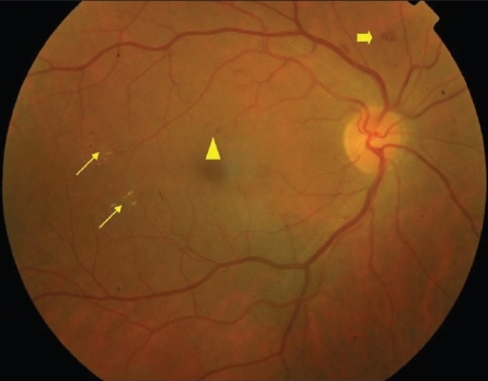
Example of non-proliferative diabetic retinopathy (NPDR): Thin arrows: hard exudates; Thick arrow: blot intra-retinal hemorrhage; Triangle: microaneurysm. (Click on image for source.)

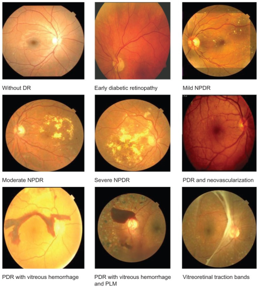
Some (sub)types of diabetic retinopathy. The competition grouped some together to get 5 ordered classes. (Click on image for source.)

Now let’s look at it as someone who simply wants to try to model this problem.

You have 35126 images in the training set that look like this

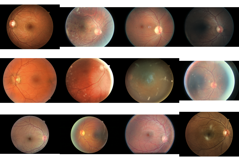
Some pseudorandom samples from the training set. Notice the black borders and different aspect ratios.

annotated by a patient id and “left” or “right” (each patient has two images, one per eye) and divided into 5 fairly unbalanced classes (per eye/image, not per patient!)

Class	Name	Number of images	Percentage
0	Normal	25810	73.48%
1	Mild NPDR	2443	6.96%
2	Moderate NPDR	5292	15.07%
3	Severe NPDR	873	2.48%
4	PDR	708	2.01%

You are asked to predict the class (thus, one of the 5 numbers) for each of the 53576 test images and your predictions are scored on the quadratic weighted kappa metric. For the public leaderboard that was updated during the competition, 20 percent of the test data was used. The other 80 percent are used to calculate the final ranking.

Not surprisingly, all my models were convolutional networks (convnets) adapted for this task. I recommend reading the well-written blogpost from the ≋ Deep Sea ≋ team that won the Kaggle National Data Science Bowl competition since there are a lot of similarities in our approaches and they provide some more/better explanation.

A small but important note: notice that 20 percent of the test images is roughly 11k images and the training set is only 35k images. Hence, the leaderboard score can actually provide some more stable scoring than only using, for example, a 90%/10% split on the training set which would result in only about a third of the size of the public leaderboard dataset used for validation. Normally I don’t like to make many submissions during a competition but because training and evaluating these models is quite time-consuming and the public leaderboard could provide some interesting and somewhat reliable information, I did try to make use of this at the end.

Also note that competing in a competition such as this requires you – unless you have a huge amount of resources and time – to interpret a stream of fairly complex and noisy data as quickly and efficiently as possible and thus, the things I have “learned” are not really tested rigorously and might even be wrong. In the same mindset, a lot of the code is written very quickly and even obvious optimisations might be postponed (or never done!) because the trade-off is not worth it, there are more immediate priorities, you don’t want to risk breaking some things, I don’t know how (to do it quickly), etc. I started working on this competition somewhere in the beginning of April because before that I was in the process of moving to London.

Overview / TL;DR

This post is written in an approximate chronological order, which might be somewhat confusing to read through at first. Therefore, I’ll try to sketch in a very concise fashion what my eventual models looked like. (It’s not completely independent of the rest of the text, which does try to provide some more explanation.)

My best models used a convolutional network with the following relatively basic architecture (listing the output size of each layer)

Nr	Name	batch	channels	width	height	filter/pool
0	Input	64	3	512	512
1	Conv	64	32	256	256	7//2
2	Max pool	64	32	127	127	3//2
3	Conv	64	32	127	127	3//1
4	Conv	64	32	127	127	3//1
5	Max pool	64	32	63	63	3//2
6	Conv	64	64	63	63	3//1
7	Conv	64	64	63	63	3//1
8	Max pool	64	64	31	31	3//2
9	Conv	64	128	31	31	3//1
10	Conv	64	128	31	31	3//1
11	Conv	64	128	31	31	3//1
12	Conv	64	128	31	31	3//1
13	Max pool	64	128	15	15	3//2
14	Conv	64	256	15	15	3//1
15	Conv	64	256	15	14	3//1
16	Conv	64	256	15	15	3//1
17	Conv	64	256	15	15	3//1
18	Max pool	64	256	7	7	3//2
19	Dropout	64	256	7	7
20	Maxout (2-pool)	64	512
21	Concat with image dim	64	514
22	Reshape (merge eyes)	32	1028
23	Dropout	32	1028
24	Maxout (2-pool)	32	512
25	Dropout	32	512
26	Dense (linear)	32	10
27	Reshape (back to one eye)	64	5
28	Apply softmax	64	5

(Where a//b in the last column denotes pool or filter size a x a with stride b x b.)

where the reshape was done to combine the representations of the two eyes belonging to the same patient. All layers were initialised with the SVD variant of the orthogonal initialisation (based on Saxe et al.) and the non-linear layers used leaky rectify units max(alpha*x, x) with alpha=0.5.

The inputs were 512x512 images which were augmented in real-time by

1. Cropping with certain probability
2. Color balance adjustment
3. Brightness adjustment
4. Contrast adjustment
5. Flipping images with 50% chance
6. Rotating images by x degrees, with x an integer in [0, 360[
7. Zooming (equal cropping on x and y dimensions)

together with their original image dimensions. Because of the great class imbalance, some classes wereoversampled to get a more uniform distribution of classes in batches. Somewhere in the middle of training this oversampling stopped and images were sampled from the true training set distribution to

1. Try to control the overfitting, which is particularly difficult when the network sees some images almost ten times more often than others.
2. Have the network fine-tune the predictions on the true class distribution.

Training was done with Stochastic Gradient Descent (SGD) and Nesterov momentum for almost 100k iterations on a loss which was a combination of a continuous kappa loss together with the cross-entropy (or log) loss:

kappalogclipped = cont_kappa + 0.5 * T.clip(log_loss, log_cutoff, 10**3)

An important part was converting the softmax probabilities for each label to a discrete prediction. Using the label with the highest probability (i.e., argmax) did quite well but is unstable and a significant improvement comes from converting these probabilities to one continuous value (by weighted sum), ranking these values and then using some boundaries to assign labels (e.g., first 10% is label 0, next 20% is label 1, etc.).

Doing all this gets you to somewhere around +0.835 with a single model.

A final good improvement then came from ensembling a few models using the mean of their log probabilities for each class, converting these to normal probabilities in [0, 1] again and using

weighted_probs = probs[:, 1] + probs[:, 2] * 2 + probs[:, 3] * 3 + probs[:, 4] * 4

to get one vector of predictions on which we can apply the ranking procedure from the previous paragraph to assign labels. A few candidate boundaries were determined using scipy’s minimize function on the kappa score of some ensembles.

The opening

The patients are always split into a training set (90%) and a validation set (10%) by stratified sampling based on the maximum label of the two eyes per patient.

Processing and augmenting

First of all, since the original images are fairly large (say, 3000x2000 pixels on average) and most contained a fairly significant black border, I started by downscaling all the images by a factor of five (without interpolation) and trying to remove most of these black borders.

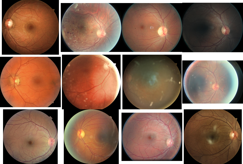
The same images from before but now the black borders are cropped.

This made it computationally much more feasible to do many augmentations: we augment the training set with seemingly similar images to increase the number of training examples.

These augmentations (transformations) were

1. Cropping with certain probability
2. Color balance adjustment
3. Brightness adjustment
4. Contrast adjustment
5. Flipping images with 50% chance
6. Rotating images by x degrees, with x an integer in [0, 360[
7. Zooming (equal cropping on x and y dimensions)

Most of these were implemented from the start. The specific ranges/parameters depend on the model (some examples can be found at the end). During training random samples are picked from the training set and transformed before queueing them for input to the network. The augmentations were done by spawning different threads on the CPU such that there was almost no delay in waiting for another batch of samples. This worked very well for most of the competition, which is why I did not spend much time trying to optimise this.

Resizing was done after the cropping and before the other transformations, because it makes some of other operations computationally way too intensive, and can be done in two ways:

1. Rescale while keeping the aspect ratio and doing a center crop on the resulting image
2. Normal bilinear rescaling, destroying the original aspect ratio

The method chosen also depends on the model. Method 1 was used a lot in the beginning, then 2 in the middle and in the end I revisited the choice again. Eventually I stuck with method 2 since my best performing models in the end used that and I did not want to have another hyperparameter to take into account, and I was afraid of losing too much information with the center crops from the first method.

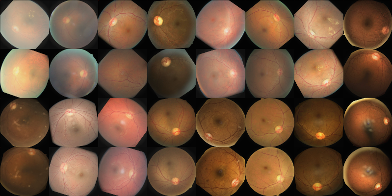
An older batch of augmented 512x512 samples as input to a network. The augmenting process went through some subtle changes since then. You can also see that the images are paired by patient but with independent augmentations (more about that later).

During the training the input is normalised by subtracting the total mean and dividing by the total standard deviation estimated on a few hundred samples before training (a pixel based normalisation was also used for a lot of models, at the moment of writing I have not figured out if there is a big difference).

The original image dimensions (before they are rescaled to a square input) are also always concatenated as features with the other dense representations (I never removed this or tested if it was of any use).

The kappa metric

The first few nets were initially trained with SGD and Nesterov momentum on the cross-entropy (or log) loss function. Thus, as a classification problem. However, the competition used the (quadratic weighted) kappa metric to score submissions and not the log loss or accuracy. The (quadratic weighted) kappa score of a class prediction y for a ground truth t can be given by the Python code (not optimised for edge cases and assuming one-hot encoded):

import numpy as np

def quadratic_kappa(y, t, eps=1e-15):
      # Assuming y and t are one-hot encoded!
      num_scored_items = y.shape[0]
      num_ratings = y.shape[1] 
      ratings_mat = np.tile(np.arange(0, num_ratings)[:, None], 
                            reps=(1, num_ratings))
      ratings_squared = (ratings_mat - ratings_mat.T) ** 2
      weights = ratings_squared / (float(num_ratings) - 1) ** 2
	
      # We norm for consistency with other variations.
      y_norm = y / (eps + y.sum(axis=1)[:, None])
	
      # The histograms of the raters.
      hist_rater_a = y_norm.sum(axis=0)
      hist_rater_b = t.sum(axis=0)
	
      # The confusion matrix.
      conf_mat = np.dot(y_norm.T, t)
	
      # The nominator.
      nom = np.sum(weights * conf_mat)
      expected_probs = np.dot(hist_rater_a[:, None], 
                              hist_rater_b[None, :])
      # The denominator.
      denom = np.sum(weights * expected_probs / num_scored_items)
	
      return 1 - nom / denom

Alternatively, for some more information about the metric, see the evaluation page of the competition. The kappa metric tries to represent the agreement between two different raters, where the score typically varies from 0 (random agreement) to 1 (complete agreement). The downside of this metric is that it is discrete – forcing you to pick only one class of the five per sample instead of allowing you to use the probabilities for each class – which necessarily gives you some more variance when evaluating models. There already is a decent amount of noise in the dataset (very questionable ground truth classifications, noisy/broken images, etc.) so there certainly was a noticeable amount of variance throughout the competition to take into account.

I only trained one or two models on the cross-entropy loss since the competition was scored on the kappa metric and I felt it was important to quickly change to a loss function closely based on this metric. Several variations of acontinuous kappa loss – you simply use your softmax prediction matrix y as input to the quadratic_kappafunction above – were tried but using only a kappa loss seemed too unstable in the beginning of training to learn well. Combining the continuous kappa with the cross-entropy loss seemed to fix this. Eventually this “kappalogclipped” loss was used

kappalogclipped = cont_kappa + 0.5 * T.clip(log_loss, log_cutoff, 10**3)

where there was an additional y_pow parameter which determined the power to which to raise the predictions before calculating the continuous kappa (squashing lower probabilities, making the predictions more discrete). This y_pow was 2 for a lot of the later experiments and has a significant influence on the model. By usingy_pow=2 the continuous kappa approximates the discrete kappa very well, which will give you some more variance in the updates. The log_cutoff determined from which point to start ignoring the log loss, this was 0.80 for most of the experiments. The scaling by 0.5 is something left behind by many other experiments with losses.

There has been a lot of discussion about optimising the kappa metric, partly because of the recent CrowdFlower Search Results Relevance competition which also used this metric to score the submissions. Most of the competitors in that competition used regression on the Mean Squared Error (MSE) objective together with somedecoding strategy to convert the continuous predictions to discrete ones. The first place winner has an excellent write-up where he compared many different methods to optimise the kappa metric and concludes that MSE together with a ranking based discretisation worked best. I also considered such an approach but since training my models took quite a while and I did not want to lose too much time testing all these different methods – and it already worked quite well! – I stuck with the kappalogclipped loss. These other losses also don’t take the distribution of the predictions into account, which I thought might be important (even though you could optimise for that after training). The kappalogclipped loss had the benefit of allowing me to easily monitor a relatively reliable kappa score during the training by using the label with the highest probability (the same argmax strategy was used for almost all the models but is revisited at the end). Also note that the fact that these labels areordered is implicitly defined by the kappa loss itself.

I did test the MSE objective very briefly at the end and got somewhat similar performance.

This was still trained with SGD with Nesterov momentum using some learning rate schedule (decreasing the learning rate 3-5 times). Most of the time some L2 regularisation on the network parameters, or weight decay, was added.

First models

My first models used 120x120 rescaled input and I stayed with that for a decent amount of time in the beginning (first 3-4 weeks). A week or so later my first real model had an architecture that looked like this (listing the output size of each layer)

Nr	Name	batch	channels	width	height	filter/pool
0	Input	32	3	120	120
1	Cyclic slice	128	3	120	120
2	Conv	128	32	120	120	3//1
3	Conv	128	16	120	120	3//1
4	Max pool	128	16	59	59	3//2
5	Conv roll	128	64	59	59
6	Conv	128	64	59	59	3//1
7	Conv	128	32	59	59	3//1
8	Max pool	128	32	29	29	3//2
9	Conv roll	128	128	29	29
10	Conv	128	128	29	29	3//1
11	Conv	128	128	29	29	3//1
12	Conv	128	128	29	29	3//1
13	Conv	128	64	29	29	3//1
14	Max pool	128	64	14	14	3//2
15	Conv roll	128	256	14	14
16	Conv	128	256	14	14	3//1
17	Conv	128	256	14	14	3//1
18	Conv	128	256	14	14	3//1
19	Conv	128	128	14	14	3//1
20	Max pool	128	128	6	6	3//2
21	Dropout	128	128	6	6
22	Maxout (2-pool)	128	512
23	Cyclic pool	32	512
24	Concat with image dim	32	514
25	Dropout	32	514
26	Maxout (2-pool)	32	512
27	Dropout	32	512
28	Softmax	32	5

(Where a//b in the last column denotes pool or filter size a x a with stride b x b.)

which used the cyclic layers from the ≋ Deep Sea ≋ team. As nonlinearity I used the leaky rectify function,max(alpha*x, x), with alpha=0.3. Layers were almost always initialised with the SVD variant of the orthogonal initialisation (based on Saxe et al.). This gave me around 0.70 kappa. However, I quickly realised that, given the grading criteria for the different classes (think of the microaneurysms which are pretty much impossible to detect on 120x120 images), I would have to use bigger input images to get anywhere near a decent model.

Something else that I had already started testing in models somewhat, which seemed to be quite critical for decent performance, was oversampling the smaller classes. I.e., you make samples of certain classes more likely than others to be picked as input to your network. This resulted in more stable updates and better, quicker training in general (especially since I was using small batch sizes of 32 or 64 samples because of GPU memory restrictions).

The middlegame

First I wanted to take into account the fact that for each patient we get two retina images: the left and right eye. By combining the dense representations of the two eyes before the last two dense layers (one of which being a softmax layer) I could use both images to classify each image. Intuitively you can expect some pairs of labels to be more probable than others and since you always get two images per patient, this seems like a good thing to do.

This gave me the basic architecture for 512x512 rescaled input which was used pretty much until the end (except for some experiments):

Nr	Name	batch	channels	width	height	filter/pool
0	Input	64	3	512	512
1	Conv	64	32	256	256	7//2
2	Max pool	64	32	127	127	3//2
3	Conv	64	32	127	127	3//1
4	Conv	64	32	127	127	3//1
5	Max pool	64	32	63	63	3//2
6	Conv	64	64	63	63	3//1
7	Conv	64	64	63	63	3//1
8	Max pool	64	64	31	31	3//2
9	Conv	64	128	31	31	3//1
10	Conv	64	128	31	31	3//1
11	Conv	64	128	31	31	3//1
12	Conv	64	128	31	31	3//1
13	Max pool	64	128	15	15	3//2
14	Conv	64	256	15	15	3//1
15	Conv	64	256	15	14	3//1
16	Conv	64	256	15	15	3//1
17	Conv	64	256	15	15	3//1
18	Max pool	64	256	7	7	3//2
19	Dropout	64	256	7	7
20	Maxout (2-pool)	64	512
21	Concat with image dim	64	514
22	Reshape (merge eyes)	32	1028
23	Dropout	32	1028
24	Maxout (2-pool)	32	512
25	Dropout	32	512
26	Dense (linear)	32	10
27	Reshape (back to one eye)	64	5
28	Apply softmax	64	5

(Where a//b in the last column denotes pool or filter size a x a with stride b x b.)

Some things that had also been changed:

1. Using higher leakiness on the leaky rectify units, max(alpha*x, x), made a big difference on performance. I started using alpha=0.5 which worked very well. In the small tests I did, using alpha=0.3 or lower gave significantly lower scores.
2. Instead of doing the initial downscale with a factor five before processing images, I only downscaled by a factor two. It is unlikely to make a big difference but I was able to handle it computationally so there was not much reason not to.
3. The oversampling of smaller classes was now done with a resulting uniform distribution of the classes. But now it also switched back somewhere during the training to the original training set distribution. This was done because initially I noticed the distribution of the predicted classes to be quite different from the training set distribution. However, this is not necessarily because of the oversampling (although you would expect it to have a significant effect!) and it appeared to be mostly because of the specific kappa loss optimisation (which takes into account the distributions of the predictions and the ground truth). It is also much more prone to overfitting when training for a long time on some samples which are 10 times more likely than others.
4. Maxout worked slightly better or at least as well as normal dense layers (but it had fewer parameters).

Visual attention

Throughout I also kept trying to find a way to work better with the high resolution input. I tried splitting the image into four (or sixteen) non-overlapping (or only slightly overlapping) squares, passing these through a smaller convnet in parallel and then combining these representations (by stacking them or pooling over them) but this did not seem to work. Something I was a little more hopeful about was using the spatial transformation layers from the Spatial Transformer Networks paper from DeepMind. The intention was to use some coarse input to make the ST-modules direct their attention to some parts of the image in higher resolution (for example, potential microaneurysms!) and hopefully they would be able to detect those finer details.

However, training this total architecture end-to-end, without initialising with a pre-trained net, was incredibly difficult at first. Even with norm constraints, lowered learning rates for certain components, smaller initialisation, etc., it was quite difficult, for one, to not have it diverge to some limiting values for the transformation parameters (which sort of makes sense). However, this might be partly because of the specific problem and/or my implementation. In the paper they also seem to work with pre-trained nets and this does seem like the way to go. Unfortunately, when I first tried this, it started overfitting quite significantly on the training set. I wish I had more time to explore this but since my more basic networks already worked so well and seemed to still allow for a decent amount of improvement, I had to prioritise those.

Some small things I have learned:

1. In general I found it is hard to have different “networks” competing with each other in one big architecture. One tends to smother the other. Even when both were initialised with some trained network. This is possibly partly because of my L2 regularisation on the network weights. I had to keep track of the activations of certain layers during training to make sure this didn’t happen.
2. It wasn’t really mentioned anywhere in the paper but I used a sort of normalisation of my transformation parameters for the ST-modules using some sigmoid.
3. I think some parts of the network might still need to be fixed (i.e., fixing the parameters) during training to get it working.

In general, I think these layers are very interesting but they certainly didn’t seem that straightforward to me. However, this might be partially because of this specific problem.

The endgame

In the last two to three weeks I was trying to wrap up any (very) experimental approaches and started focusing on looking more closely at the models (and their predictions) to see where I could maybe still improve. The “basic architecture” from the previous section barely changed for more than a month and most of my improvements came from optimising the learning process. My best (leaderboard) score (of about 0.828, which was top 3 for a few weeks) three weeks before the end of the competition came from a simple log mean ensemble from 2-3 models scoring individually around 0.82.

Camera artifacts

When looking at the two images of certain patients next to each other I noticed something which is harder to see when looking at single images: camera artifacts.

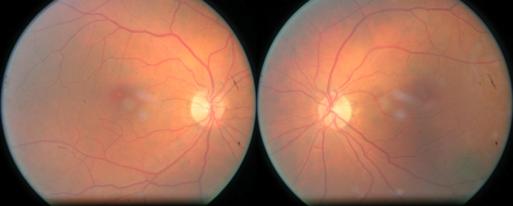
Sample camera artifacts: tiny black dots on the outer left center and bigger black spots and stripes on the outer right.

Sometimes they can even resemble microaneurysms (well, they can be tiny black dots, the size of a microaneurysm) and it can be very hard to distinguish between the two unless you have the other image. Even more, these artifacts seemed to be fairly common as well! The problem is: it is very unlikely my models at the time would be able to figure this out because

1. Although they take both eyes into account by merging the dense representations, these are very high level representations (fully connected layers get rid of a lot of the spatial information, see e.g. Dosovitskiy and Brox).
2. Augmentations were done on each eye separately, independent of patient. I did have a “paired transformations” option but at the time I did not see any big improvements using that.

One thing I tried to take this into account was to merge the outputs of the first convolutional or pooling layer for each of the two eyes (or maybe even the input layer). Then theoretically the convolutional layer could be able to detect similar patterns in the left and right eye. However, then I felt I was reducing the input space way too much after the merging (which was – and had to be – done in the first few layers) and thus, I instead took the outputsa and b from the output of some layer (for the two eyes of a patient) and replaced them with ab and ba bystacking them on the channel dimension (instead of simply replacing them both by ab). This way the net still had access to the other low level representations but I was not losing half the input space.

Unfortunately this did not seem to help that much and I was running out of time such that I put this aside.

Pseudo-labeling

Nearer to the end of the competition I also started testing the clever pseudo-labeling idea from the ≋ Deep Sea ≋ team which uses the predictions from other (ensembles of) models on the test set to help guide or regularise new models. Essentially, during training I added some test images to the batches, such that on average roughly 25% of the batch was comprised of images from the test set, together with the softmax predictions for those images from my best ensemble. This probably helped to push me to about 0.83 for a single model.

Better decoding

For a long time I simply used the class with the highest probability from my softmax output as my prediction (i.e.,argmax). Even though this allowed me to get this far, it was obvious that this method is quite unstable since it doesn’t take the magnitude of the (other) probabilities into account, only their size relative to each other. To get around that, I used a similar ranking decoding strategy as was used by some people in the CrowdFlower Search Results Relevance competition: first we convert the probabilities from the softmax output to one value by weighing each probability by the class label {0, 1, 2, 3, 4}

weighted_probs = probs[:, 1] + probs[:, 2] * 2 + probs[:, 3] * 3 + probs[:, 4] * 4

Next we rank the weighted probabilities from low to high and try to find the most optimal boundaries [x_0, x_1, x_2, x_3] to assign labels. I.e., the images with a weighted probability in [0, x_0[ we assign the label 0, the images with a weighted probability in [x_0, x_1[ we assign the label 1, etc. I used scipy’s minimize function to quickly find some boundaries that optimise the kappa score on the train set of some ensemble. This probably could have been optimised better but I did not want to overtune and have the risk of badly overfitting.

This helped quite a bit, pushing some of my single models from 0.83 to 0.835. However, I was kind of surprised that changing the prediction distribution quite significantly with different boundaries did not result in bigger differences in scores.

Error distribution

Something that stood out was the fact that the models were highly variable on the validation sets. Although this was mostly because of the discrete metric, the noise in the dataset itself and my small validation set, I still wanted to try to find out more. If you look at the quadratic_kappa metric/loss above you can see that it is determined by two matrices: nom and denom. The kappa score is then given by 1 - sum(nom) / sum(denom). Hence, you want to minimise the nom sum and maximise the denom sum. The denominator denom is fairly stable and captures the distributions of the predictions and the targets. The nominator nom is the one which will give us the most insight into our model’s predictions. Let’s look at the nom and denom for some random well-performing model (+0.82 kappa) when I was using the simple argmax decoding:

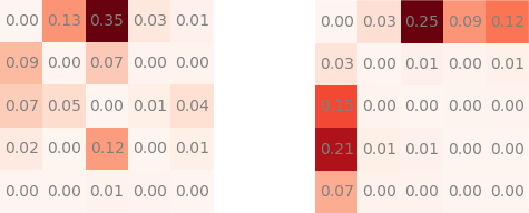
Normalised nom (left) and denom (right) for some well performing model with highest probability decoding (+0.82 kappa). Position (i, j) = predicted i for true label j.

Whereby the matrices are normalised and show the percentage of the total sum located in that position. You immediately notice something: the error is almost dominated by the errors of predicting class 0 when it was really class 2 (i.e., you predict a normal eye but it is really a moderate NPR eye). Initially this gives you some hope, since you think you should be able to bring down some misclassifications which are 2 classes apart and they would have an important impact on your score. However, the problem with this, and in general, was that the ground truth was not sure at all (since I’m not an ophthalmologist, not even a doctor!) and some really questionable classifications had already come to light.

Because the other ranking decoding strategy is only applied after training and was done quite late in the competition, I don’t have any error distribution pictures for those yet. But I do remember the nom behaving quite similarly and most of the error (30-40%) coming from predicting class 0 when it was really class 2.

Ensembling

A good improvement then came from ensembling a few models using the mean of their log probabilities for each class, converting these to normal probabilities in [0, 1] again and using the ranking decoding strategy from one of the previous paragraphs to assign labels to the images. A few candidate boundaries were determined usingscipy’s minimize function on the kappa score of some ensembles. Doing this on the best models at the time pushed my models to +0.84.

Other (not) tried approaches and papers

Some other things that did not seem to work (well enough):

• Batch Normalisation: although it allowed for higher learning rates, it did not seem to speed up training all that much. (But I do believe the training of convnets should be able to be much faster than it is now.)
• Other types of updates (e.g., ADAM): especially with the special loss based on the kappa metric I was not able to get it working well.
• Remove pooling layers: replacing all the 3//2 (pool size 3x3 and stride 2x2) max pooling layers with a 3//2convolutional layer made the training quite a bit slower but more importantly seemed to have pretty bad performance. (I was more hopeful about this!)
• PReLU: tried it only briefly but it seemed to only worsen performance / result in (more) overfitting.
• Using 2//2 max pooling instead of 3//2 in the hope of being able to distinguish finer details better (since, for example, microaneurysms are most of the time located closely to some vessel).
• Several architecture changes: more convolutional layers after the first, second or third pooling layer, bigger filter size in the first layer, replace the first 7//2 convolutional and 3//2 pooling layer by two 5//2 convolutional layers, etc. But it did not seem to help that much and I was struggling with the variance of the models.
• Second level model: at the very, very end I tried using second level models (such as ridge regression, Lasso, etc.) on the softmax outputs of many different models (instead of just using a log mean ensemble). Unfortunately, in my case, it was too messy to do this at the last minute with many models with small and different validation sets. But I would expect it to potentially work really well if you are able to regularise it enough.

Some things I haven’t tried:

• Specialist networks: makes everything much more complicated and there was still the problem of some classes being very small. I also wasn’t sure at all that it would have helped.
• Higher resolution input: 512x512 was about the limit for networks that could train in 1-2 days on a GTX 980. One of the bigger bottlenecks then actually became the augmentation. I estimated from looking at some images (and hoped) that 512x512 would be able to capture most of the information.
• Implementing one of the many more manual approaches: there were many papers reviewing the different approaches tried in the literature for detecting diabetic retinopathy on eye images and most of them were quite manual (constructing several filters and image processing pipelines to extract features). I believe(d) quite firmly that a convnet should be able to do all of that (and more) but supplementing the network with some of these manual approaches might have been helpful since you could simply run it only once on higher resolution input (maybe helping you detect, for example, microaneurysms). However, I couldn’t bring myself to do all this manual image processing and wanted a more elegant solution.
• Unsupervised training: it would have been a bit of a gamble since I haven’t read that many recent experiences where unsupervised training was very helpful and it would have taken a lot of time. I certainly wanted to use the test set and was more than happy with the pseudo-labeling approach.
• Multiple streams / scales / crops: I felt I had more immediate problems to overcome and this would have made the model too big (for my resources).

I have read quite a few papers (and skimmed a lot more) and even though some of them were very interesting, I was quite limited in time and resources to try them all out. Some I have read and found interesting (not necessarily directly related to this competition):

• Efficient Multiple Instance Convolutional Neural Networks for Gigapixel Resolution Image Classification: in the paper they iteratively select discriminative patches, patches whose hidden label equals the true label of the image, from a gigapixel resolution image and train a convnet on them. I decided the retina images did not need to be that high res to capture almost all the low level information to have to do something like this (I would guess maximum 1024x1024, probably smaller, which is still very big but more doable). It also felt a little unsuitable for these eye images that have so many different types of low level information (not the best explanation).
• Multiple Object Recognition with Visual Attention and Spatial Transformer Networks: these are two different methods to have visual attention on images: the first uses recurrent nets, the second normal, end-to-end convnets. This was all when I was searching for a way to be able to work with higher resolution images.
• Inverting Convolutional Networks with Convolutional Networks, Visualizing and Understanding Convolutional Networks and Object Detectors Emerge in Deep Scene CNNs: all of these papers try to deduce what kind of information each layer holds, how well you can reconstruct the original image just from this information and some try to see how invariant this information is under certain transformations of the original image. If you’ve heard or read about DeepDream (kind of hard not to have), there are some related things going on in the first paper but more theoretical. The more direct inspiration for DeepDream was the paper Deep Inside Convolutional Networks: Visualising Image Classification Models and Saliency Maps which is also very interesting!

Conclusion

The actual process was quite a bit more lengthy and chaotic (especially at the end) but hopefully this captures the most important elements of my competition experience. All in all, a relatively basic architecture was able to achieve top scores in this competition. Nevertheless, the predictions always felt quite “weak” and my feeling is that there is still quite a bit of room for improvement. Without a doubt the biggest difficulty for me was dealing with the large amount of variance resulting from

1. the noisy labels
2. the extremely small classes (the two highest gradings together represent less than 5% of the samples!)
3. the discrete metric which then very heavily punishes extreme misclassifications (and this in combination with the previous point!)

Maybe I should have worked harder on taking 2. into account, although, when checking the misclassifications of my models, I still felt that 1. was a very significant problem as well. It would be very interesting (and important!) to get some scores of other (human) expert raters.

In hindsight, optimising learning on the special kappa metric seemed to be much more important than optimising the architecture and I did lose a lot of time trying to work with some more special architectures because I thought they might be needed to be able to finish high enough. It is also possible that the MSE objective was the better choice for this competition. I tested it briefly at the end and the performance seemed somewhat similar but I would expect it to be more stable than using my kappalogclipped loss. I should also have explored different train/validation splits instead of always using 90%/10% splits. This possibly could have made evaluating the models more stable.

Personally, I very much enjoyed the competition. I learned a lot, am left with a whole bunch of ideas to work on and many pages of ugly code to rework. Hopefully next time I can compete together with other smart, motivated people since I miss having those interactions and doing everything on my own while also working a full time job was quite challenging and exhausting! Congratulations to the winners and all the people who contributed!

Also, when comparing results from this competition to other approaches or software, take into account that it does not necessarily make any sense because they may be training and/or evaluating on different datasets!

Code, models and example activations

Everything was trained on a NVIDIA GTX 980 in the beginning; this was the GPU for the desktop I was also working on, which wasn’t ideal. Therefore, later I also tried using the GRID K520 on AWS (even though it was at least two times slower). The code is based on the code from the ≋ Deep Sea ≋ team that won the Kaggle National Data Science Bowl competition and uses mostly Lasagne (which uses Theano). Models (including static and learned parameters and data from the training) were dumped via cPickle and a quickly written script was used to produce images for each of these dumps summarising the model and its performance. For example:

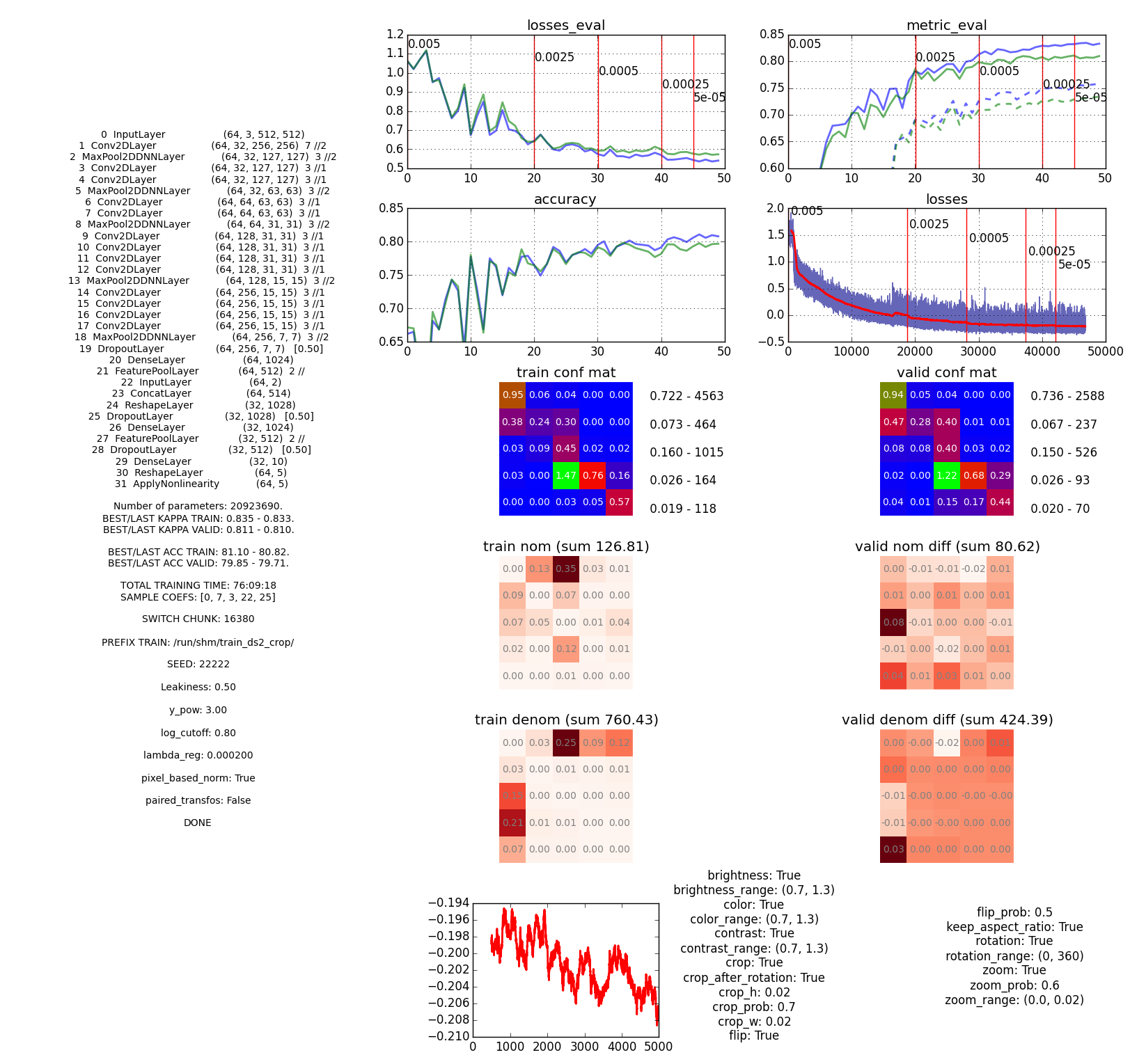
Example of a model image. It isn't the prettiest but it has almost all the information I need. This model got about0.824 on the public leaderboard. The long training time is mostly because of AWS. (Click to enlarge.)

This way it was much easier to compare models and keep track of them. (This is just an example to give you an idea of one method I used to compare models. If you are curious about the specifics, you can find all the information in the code itself.)

Example activations for one of the better models with the basic 512x512 architecture (each vertical block represents the output of one channel of the layer):

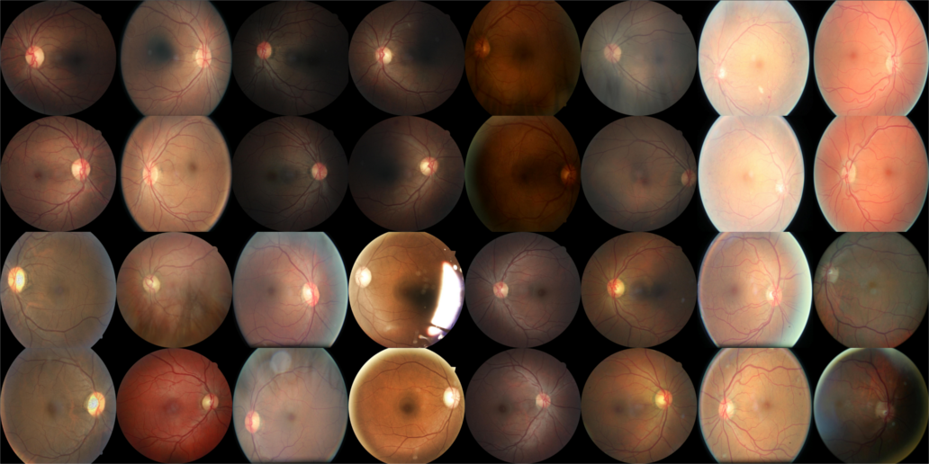
Input layer without augmentations and normal rescaling. Labels (from left to right, up to down): 0, 0, 0, 2, 1, 0, 4, 0 -- 1, 0, 0, 2, 2, 0, 4, 0 -- 0, 0, 0, 0, 0, 2, 2, 0 -- 0, 0, 0, 0, 0, 2, 3, 0. Click for larger image (4.5MB).

First layer, 7//2 convolutional layer activations. Click for larger image (24MB).

Second layer, 3//2 pooling layer activations. Click for larger image (19MB).

Third layer, 3//1 convolutional layer activations. Click for larger image (20MB).

Fourth layer, 3//1 convolutional layer activations. Click for larger image (21MB).

Fifth layer, 3//2 pooling layer activations. Click for larger image (17MB).

I also want to publish some models with all the learned parameters. To be continued.

Thanks

I would like to thank Kaggle, California Healthcare Foundation and EyePACS for organising and/or sponsoring this challenging competition. Also many thanks to the wonderful developers and contributors of Theano and Lasagnefor their continuous effort on these libraries.