mathworks社区中的这个资料还是值得一说的。
1 openExample('mpc/mpccustomqp')
我们从几个角度来解析两者关系,简单的说就是MPC是带了约束的LQR.
下面我们从代码的角度解析这个问题:
1, 定义被控系统:
1 A = [1.1 2; 0 0.95];
2 B = [0; 0.0787];
3 C = [-1 1];
4 D = 0;
5 Ts = 1;
6 sys = ss(A,B,C,D,Ts);
7 x0 = [0.5;-0.5]; % initial states at [0.5 -0.5]
2,设计无约束LQR:

1 Qy = 1;
2 R = 0.01;
3 K_lqr = lqry(sys,Qy,R);
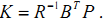
3, 运行仿真闭环结果:
1 t_unconstrained = 0:1:10;
2 u_unconstrained = zeros(size(t_unconstrained));
3 Unconstrained_LQR = tf([-1 1])*feedback(ss(A,B,eye(2),0,Ts),K_lqr);
4 lsim(Unconstrained_LQR,'-',u_unconstrained,t_unconstrained,x0);
5 hold on;
4,设计MPC控制器:
1 %%
2 % The MPC objective function is |J(k) = sum(x(k)'*Q*x(k) + u(k)'*R*u(k) +
3 % x(k+N)'*Q_bar*x(k+N))|. To ensure that the MPC objective function has the
4 % same quadratic cost as the infinite horizon quadratic cost used by LQR,
5 % terminal weight |Q_bar| is obtained by solving the following Lyapunov
6 % equation:
7 Q = C'*C;
8 Q_bar = dlyap((A-B*K_lqr)', Q+K_lqr'*R*K_lqr);
9
10 %%
11 % Convert the MPC problem into a standard QP problem, which has the
12 % objective function |J(k) = U(k)'*H*U(k) + 2*x(k)'*F'*U(k)|.
13 Q_hat = blkdiag(Q,Q,Q,Q_bar);
14 R_hat = blkdiag(R,R,R,R);
15 H = CONV'*Q_hat*CONV + R_hat;
16 F = CONV'*Q_hat*M;
17
18 %%
19 % When there are no constraints, the optimal predicted input sequence U(k)
20 % generated by MPC controller is |-K*x|, where |K = inv(H)*F|.
21 K = HF;
22
23 %%
24 % In practice, only the first control move |u(k) = -K_mpc*x(k)| is applied
25 % to the plant (receding horizon control).
26 K_mpc = K(1,:);
27
28 %%
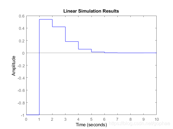
29 % Run a simulation with initial states at [0.5 -0.5]. The closed-loop
30 % response is stable.
31 Unconstrained_MPC = tf([-1 1])*feedback(ss(A,B,eye(2),0,Ts),K_mpc);
32 lsim(Unconstrained_MPC,'*',u_unconstrained,t_unconstrained,x0)
33 legend show
到这里,完全可以说明,在无约束前提下,两种方法是一致的:
1 K_lqr =
2
3     4.3608   18.7401
4
5
6 K_mpc =
7
8     4.3608   18.7401
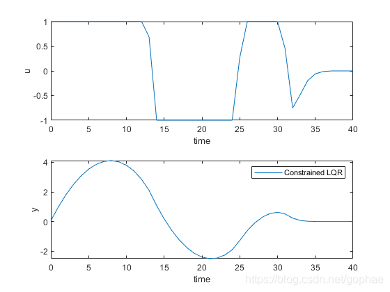
5,对LQR施加约束:
 1 x = x0;
 2 t_constrained = 0:40;
 3 for ct = t_constrained
 4 uLQR(ct+1) = -K_lqrx;
 5 uLQR(ct+1) = max(-1,min(1,uLQR(ct+1)));
 6 x = Ax+BuLQR(ct+1);
 7 yLQR(ct+1) = Cx;
 8 end
 9 figure
10 subplot(2,1,1)
11 plot(t_constrained,uLQR)
12 xlabel(‘time’)
13 ylabel(‘u’)
14 subplot(2,1,2)
15 plot(t_constrained,yLQR)
16 xlabel(‘time’)
17 ylabel(‘y’)
18 legend(‘Constrained LQR’)
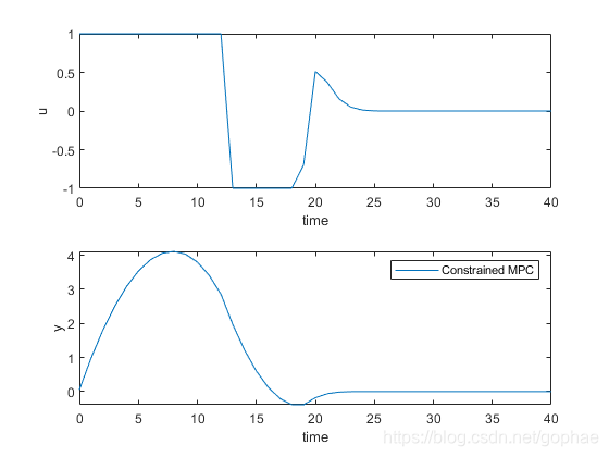
6,对MPC施加约束:
 1 %% MPC Controller Solves QP Problem Online When Applying Constraints
 2 % One of the major benefits of using MPC controller is that it handles
 3 % input and output constraints explicitly by solving an optimization
 4 % problem at each control interval.
 5 %
 6 % Use the built-in KWIK QP solver, |mpcqpsolver|, to implement the custom
 7 % MPC controller designed above. The constraint matrices are defined as
 8 % Ac*x>=b0.
 9 Ac = -[1 0 0 0;...
10       -1 0 0 0;...
11        0 1 0 0;...
12        0 -1 0 0;...
13        0 0 1 0;...
14        0 0 -1 0;...
15        0 0 0 1;...
16        0 0 0 -1];
17 b0 = -[1;1;1;1;1;1;1;1];
18
19 %%
20 % The |mpcqpsolver| function requires the first input to be the inverse of
21 % the lower-triangular Cholesky decomposition of the Hessian matrix H.
22 L = chol(H,'lower');
23 Linv = Leye(size(H,1));
24
25 %%
26 % Run a simulation by calling |mpcqpsolver| at each simulation step.
27 % Initially all the inequalities are inactive (cold start).
28 x = x0;
29 iA = false(size(b0));
30 opt = mpcqpsolverOptions;
31 opt.IntegrityChecks = false;
32 for ct = t_constrained
33     [u, status, iA] = mpcqpsolver(Linv,F*x,Ac,b0,[],zeros(0,1),iA,opt);
34     uMPC(ct+1) = u(1);
35     x = A*x+B*uMPC(ct+1);
36     yMPC(ct+1) = C*x;
37 end
38 figure
39 subplot(2,1,1)
40 plot(t_constrained,uMPC)
41 xlabel('time')
42 ylabel('u')
43 subplot(2,1,2)
44 plot(t_constrained,yMPC)
45 xlabel('time')
46 ylabel('y')
47 legend('Constrained MPC')
转载:https://blog.csdn.net/gophae/article/details/104546805/