利用Python进行数据分析这本书,介绍了高效解决各种数据分析问题的Python语言和库,结合其他学习资源集中总结一下Python数据分析相关库的知识点。
数据分析相关库
(1) NumPy
NumPy(Numerical Python)是Python科学计算的基础包,支持大量的维度数组与矩阵运算,此外也针对数组运算提供大量的数学函数库。也就是说,Numpy是一个运行速度非常快的数学库,主要功能包括:
- 快速高效的多维数组对象ndarray
- 用于对数组执行元素级计算以及直接对数组执行数学运算的函数
- 用于读写硬盘上基于数组的数据集的工具
- 线性代数运算、傅里叶变换,以及随机数生成
- 用于将C、C++、Fortran代码集成到python的工具
NumPy最重要的特点是其N维数组对象(ndarray),该对象是一个快速而良好的大数据集容器,需要掌握数组对象的常用语法。
import numpy as np
data = np.array([1, 2, 3, 4, 5])
print (data)

#输出 [1 2 3 4 5]
print (data.shape) #shape 表示各维度大小的元组
#输出
(5,)   #一维数组

print (data.ndim) #ndim 维度大小
#输出
1
print (data.size) #size 表示多少元素
#输出
5
print (data.dtype) #dtype 数组的数据类型
#输出
int32
print(np.zeros((2,3))) #创建指定长度的全0数组
#输出
[[0. 0. 0.]
 [0. 0. 0.]]
print (np.ones((3,6))) #创建指定长度的全1数组
#输出
[[1. 1. 1. 1. 1. 1.]
 [1. 1. 1. 1. 1. 1.]
 [1. 1. 1. 1. 1. 1.]]
print (np.empty((3,2,3))) #创建一个没有任何值的数组
#输出
[[[1. 1. 1.]
  [1. 1. 1.]]

 [[1. 1. 1.]
  [1. 1. 1.]]

 [[1. 1. 1.]
  [1. 1. 1.]]]
print (np.arange(0,10,2)) #arrange是Python内置函数range的数组版
#输出
[0 2 4 6 8]
print (np.arange(15).reshape(3,5)) #reshape 转换成3*5的矩阵
#输出
[[ 0  1  2  3  4]
 [ 5  6  7  8  9]
 [10 11 12 13 14]]
print (np.arange(10)[5:8]) #切片
#输出
[5 6 7]
print (np.random.random((2,3))) #numpy.random模块对Python内置的random进行补充
#输出
[[0.63545712 0.36970827 0.27986446]
 [0.49481143 0.76131889 0.65610538]]

a = np.array([(1, 2, 3), (4, 5, 6), (7, 8, 9)])

a
Out[8]:
array([[1, 2, 3],
       [4, 5, 6],
       [7, 8, 9]])

a[0], a[-1]     #二维数组索引 取第1行、最后1行
Out[9]: (array([1, 2, 3]), array([7, 8, 9]))

a[:, 1]    #二维数组切片 取第2列
Out[10]: array([2, 5, 8])

a[1:3, :]    #二维数组切片 取第2、3行
Out[11]:
array([[4, 5, 6],
       [7, 8, 9]])

a
Out[15]:
array([[ 0.34927643,  0.56167914],
       [ 0.53429451,  0.38356559],
       [ 0.37718082,  0.32356081]])

a.ravel()     #展平数组
Out[16]:
array([ 0.34927643,  0.56167914,  0.53429451,  0.38356559,  0.37718082,
        0.32356081])

a = np.random.randint(10, size=(3,3))

b = np.random.randint(10, size=(3,3))

a, b
Out[19]:
(array([[0, 5, 6],
        [3, 1, 5],
        [5, 2, 1]]), array([[8, 3, 4],
        [6, 1, 1],
        [8, 5, 5]]))

np.vstack((a, b))    #垂直拼合数组
Out[20]:
array([[0, 5, 6],
       [3, 1, 5],
       [5, 2, 1],
       [8, 3, 4],
       [6, 1, 1],
       [8, 5, 5]])

np.hstack((a, b))  #水平拼合数组
Out[21]:
array([[0, 5, 6, 8, 3, 4],
       [3, 1, 5, 6, 1, 1],
       [5, 2, 1, 8, 5, 5]])

np.hsplit(a, 3)   #沿横轴分割数组
Out[22]:
[array([[0],
        [3],
        [5]]), array([[5],
        [1],
        [2]]), array([[6],
        [5],
        [1]])]

np.vsplit(a, 3)   #沿纵轴分割数组
Out[23]: [array([[0, 5, 6]]), array([[3, 1, 5]]), array([[5, 2, 1]])]

a = np.array(([1, 4, 3], [6, 2, 9], [4, 7, 2]))

a
Out[25]:
array([[1, 4, 3],
       [6, 2, 9],
       [4, 7, 2]])

np.min(a, axis=1)    #返回每行最小值
Out[26]: array([1, 2, 2])

np.max(a, axis = 0)   #返回每列最大值
Out[27]: array([6, 7, 9])

np.argmax(a, axis=0)  #返回每列最大值索引
Out[28]: array([1, 2, 1], dtype=int64)

np.argmin(a, axis=1)  #返回每行最小值索引
Out[29]: array([0, 1, 2], dtype=int64)

#数组统计

np.median(a, axis=0)    # 统计数组各列的中位数
Out[30]: array([ 4.,  4.,  3.])

np.mean(a, axis=1)     #统计数组各行的算术平均值
Out[31]: array([ 2.66666667,  5.66666667,  4.33333333])

np.average(a, axis=0)   #统计数组各列的加权平均值
Out[32]: array([ 3.66666667,  4.33333333,  4.66666667])

np.var(a, axis=1)      #统计数组各行的方差
Out[33]: array([ 1.55555556,  8.22222222,  4.22222222])
使用 Z-Score 标准化算法对数据进行标准化处理,Z-Score 标准化公式
#Z-Score标准化公式
import numpy as np
#根据公式定义函数
def zscore(x, axis = None):
    xmean = x.mean(axis=axis, keepdims=True)
    xstd = np.std(x, axis=axis, keepdims=True)
    zscore = (x-xmean)/xstd
    return zscore

#生成随机数据
Z = np.random.randint(10, size=(5,5))
print(Z)
print(zscore(Z))
#输出
[[1 2 2 6 2]
 [0 0 4 0 1]
 [4 0 9 2 1]
 [3 7 1 5 3]
 [4 2 4 5 2]]
[[-0.78935222 -0.35082321 -0.35082321  1.40329283 -0.35082321]
 [-1.22788123 -1.22788123  0.52623481 -1.22788123 -0.78935222]
 [ 0.52623481 -1.22788123  2.71887986 -0.35082321 -0.78935222]
 [ 0.0877058   1.84182184 -0.78935222  0.96476382  0.0877058 ]
 [ 0.52623481 -0.35082321  0.52623481  0.96476382 -0.35082321]]
使用 Min-Max 标准化算法对数据进行标准化处理,Min-Max 标准化公式
#Min-Max 标准化公式
import numpy as np
def min_max(x, axis=None):
    min = x.min(axis=axis, keepdims=True)
    max = x.max(axis=axis, keepdims=True)
    result = (x-min)/(max-min)
    return result
Z = np.random.randint(10, size=(5, 5))
print(Z)
print(min_max(Z))

#输出

[[3 8 3 2 7]
 [9 2 6 3 4]
 [4 5 9 0 1]
 [6 6 4 1 4]
 [1 2 2 1 6]]
[[ 0.33333333  0.88888889  0.33333333  0.22222222  0.77777778]
 [ 1.          0.22222222  0.66666667  0.33333333  0.44444444]
 [ 0.44444444  0.55555556  1.          0.          0.11111111]
 [ 0.66666667  0.66666667  0.44444444  0.11111111  0.44444444]
 [ 0.11111111  0.22222222  0.22222222  0.11111111  0.66666667]]
使用 L2 范数对数据进行标准化处理,L2 范数计算公式:
#L2范数标准化
import numpy as np
def l2_normalize(v, axis=-1, order=2):
    l2 = np.linalg.norm(v, ord=order, axis=axis, keepdims=True)
    l2[l2==0] = 1
    return v/l2
Z = np.random.randint(10, size=(5,5))
print(Z)
print(l2_normalize(Z))
#输出
[[2 0 2 0 4]
 [8 1 9 2 1]
 [8 6 4 2 5]
 [4 4 7 5 5]
 [3 6 3 1 0]]
[[ 0.40824829  0.          0.40824829  0.          0.81649658]
 [ 0.65103077  0.08137885  0.73240961  0.16275769  0.08137885]
 [ 0.66436384  0.49827288  0.33218192  0.16609096  0.4152274 ]
 [ 0.34948162  0.34948162  0.61159284  0.43685203  0.43685203]
 [ 0.40451992  0.80903983  0.40451992  0.13483997  0.        ]]
总结:ndarray是一个通用的同构数据多维容器,也就是说,其中的所有元素必须是相同类型的。除了上面介绍的numpy的用法以外,numpy同样支持数组的各类计算,包括索引、点积、转置,快速的元素级数组函数(abs() sqrt() exp() add() maximun())、逻辑运算、数组统计方法(mean() sum() std() var())、排序(sort)和集合、线性代数函数(dot() diag() trace() det() eig()) 等。
(2) pandas
pandas提供了使数据分析工作变得更快更简单的高级数据结构和操作工具。pandas兼具Numpy高性能的数组计算功能以及电子表格和关系型数据(如SQL)灵活的数据处理能力。它是基于NumPy构建的,让以NumPy为中心的应用变得更加简单。Pandas 的数据结构:Pandas 主要有 Series(一维数组),DataFrame(二维数组),Panel(三维数组),Panel4D(四维数组),PanelND(更多维数组)等数据结构。其中 Series 和 DataFrame 应用的最为广泛。
- Series 是一维带标签的数组,它可以包含任何数据类型。包括整数,字符串,浮点数,Python 对象等。Series 可以通过标签来定位。 即Series基本结构为
pandas.Series(data=None, index=None) - DataFrame 是二维的带标签的数据结构,可以通过标签来定位数据。这是 NumPy 所没有的。即DataFrame基本结构为
pandas.DataFrame(data=None, index=None, columns=None)
#创建Series 数据类型
#方式1 从列表创建 Series
import pandas as pd
obj = pd.Series([4, 7, -5, 3])
print (obj)

#输出
0    4
1    7
2   -5
3    3
dtype: int64

#方式2 从 Ndarray 创建 Series

import numpy as np
import pandas as pd
n = np.random.randn(5)
index = ['a', 'b', 'c', 'd', 'e']
s = pd.Series(n, index=index)
print(s)
#输出
a   -1.110084
b   -0.141548
c    0.177586
d   -0.437167
e   -1.348287
dtype: float64

#方式3 从字典创建 Series


import pandas as pd
d = {'a':1, 'b':2, 'c':3, 'd':4, 'e':5}
s = pd.Series(d)
print(s)
#输出
a    1
b    2
c    3
d    4
e    5
dtype: int64
DataFrame是一个表格型的数据结构,它含有一组有序的列,每列可以是不同的值类型。DataFrame既有行索引也有列索引,可以看做是由Series组成的字典(共用同一个索引),另外,DataFrame中面向行和面向列的操作基本上是平衡的。构建DataFrame的办法有很多,最常用的是直接传入一个由等长列表或NumPy数组组成的字典。
- 创建 DataFrame 数据类型
#方法1 通过字典数组创建 DataFrame
import pandas as pd
data = {'name':['Jame','Lily','Noe'],'age':[21,19,17]}
frame = pd.DataFrame(data)
print (frame)
#输出
   age  name
0   21  Jame
1   19  Lily
2   17   Noe
- 从np.array 转换为 pd.DataFrame
#方式2 通过 NumPy 数组创建 DataFrame
import pandas as pd
data = np.array([('Jame',21),('Lily',19),('Noe',17)])
frame = pd.DataFrame(data,index = range(1,4),columns=['name','age'])
print (frame)
#输出
  name age
1  Jame  21
2  Lily  19
3   Noe  17
(3) matplotlib
绘图是数据分析工作中的重要部分,可以帮助我们找到异常值、必要的数据转换、得出有关模型的Idea等,Python有许多可视化工具,主要介绍使用 Matplotlib 绘图的方法和技巧。
使用 Matplotlib 提供的面向对象 API,需要导入 pyplot 模块,简称为 plt,pyplot 模块是 Matplotlib 最核心的模块,几乎所有样式的 2D 图形都是经过该模块绘制出来的。举例,通过 1 行代码绘制2D图形
from matplotlib import pyplot as plt
plt.plot([2, 3, 4, 5, 6, 7, 8, 9, 10, 11, 12, 13, 14, 15, 16],
         [1, 2, 3, 2, 1, 2, 3, 4, 5, 6, 5, 4, 3, 2, 1])
另有 plt.bar([1, 2, 3], [1, 2, 3]) 绘制柱形图, plt.scatter() 绘制散点图, plt.pie() 绘制饼状图等
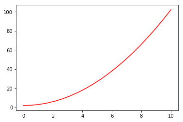
此外,Matplotlib提供兼容MATLAB API ,需要导入pylab模块
import numpy as np
from matplotlib import pylab
x = np.linspace(0, 10, 20)     #使用 NumPy 生成随机数据
y = x*x +2
pylab.plot(x, y, 'r')
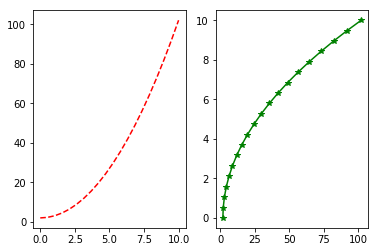
如果要绘制子图,就可以使用 subplot 方法绘制子图
pylab.subplot(1, 2, 1)
pylab.plot(x, y, 'r--')
pylab.subplot(1, 2, 2)
pylab.plot(y, x, 'g*-')
上面讲到使用 Matplotlib 中的 pyplot 模块绘制简单的 2D 图像。其实,Matplotlib 也可以绘制 3D 图像,与二维图像不同的是,绘制三维图像主要通过 mplot3d 模块实现。
mplot3d 模块下主要包含 4 个大类:
mpl_toolkits.mplot3d.axes3d()mpl_toolkits.mplot3d.axis3d()mpl_toolkits.mplot3d.art3d()mpl_toolkits.mplot3d.proj3d()
其中,axes3d()下面主要包含了各种实现绘图的类和方法。axis3d()主要是包含了和坐标轴相关的类和方法。art3d()包含了一些可将 2D 图像转换并用于 3D 绘制的类和方法。proj3d()中包含一些零碎的类和方法。
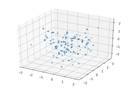
一般,用到最多的就是 mpl_toolkits.mplot3d.axes3d() 下面的 mpl_toolkits.mplot3d.axes3d.Axes3D() 类,例如,绘制三维散点图
import numpy as np
from mpl_toolkits.mplot3d import Axes3D
import matplotlib.pyplot as plt

#x y z是0到1之间的100个随机数
x = np.random.normal(0, 1, 100)
y = np.random.normal(0, 1, 100)
z = np.random.normal(0, 1, 100)
fig = plt.figure()
ax = Axes3D(fig)
ax.scatter(x, y, z)
(4) SciPy
SciPy(Scientific Python)是开源的Python算法库和数学工具包。SciPy 包含的模块有最优化、线性代数、积分、插值、特殊函数、快速傅里叶变换、信号处理和图像处理、常微分方程求解和其他科学与工程中常用的计算。
- 常量模块
为了方便科学计算,SciPy 提供了一个叫 scipy.constants 模块,该模块下包含了常用的物理和数学常数及单位。
from scipy import constants

constants.pi    #数学中的圆周率
Out[47]: 3.141592653589793

constants.golden    #黄金分割常数
Out[48]: 1.618033988749895

constants.c, constants.speed_of_light     #真空中的光速、普朗克系数
Out[49]: (299792458.0, 299792458.0)

constants.h, constants.Planck
Out[50]: (6.62607004e-34, 6.62607004e-34)
- 线性代数
线性代数是科学计算中最常涉及到的计算方法之一,SciPy 中提供了各种线性代数计算函数。这些函数基本都放置在模块 scipy.linalg 下方。又大致分为:基本求解方法,特征值问题,矩阵分解,矩阵函数,矩阵方程求解,特殊矩阵构造等。
import numpy as np

from scipy import linalg

linalg.inv(np.matrix([[1, 2], [3, 4]]))   #矩阵的逆,用到 scipy.linalg.inv 函数
Out[53]:
array([[-2. ,  1. ],
       [ 1.5, -0.5]])

U, s, Vh = linalg.svd(np.random.randn(5, 4))    #scipy.linalg.svd 函数 ,随机矩阵完成奇异值分解

U, s, Vh
Out[55]:
(array([[-0.25343531, -0.88646496,  0.01813706,  0.3488603 ,  0.16708669],
        [-0.34041342, -0.04125014, -0.19885736, -0.65156027,  0.6467937 ],
        [ 0.57594129,  0.08312343,  0.32251328,  0.28171905,  0.69137667],
        [-0.53214652,  0.18716945,  0.82464561,  0.03584257,  0.02150823],
        [-0.45277031,  0.41296053, -0.41960887,  0.61083172,  0.27436408]]),
 array([ 2.9389141 ,  2.27087176,  1.9896549 ,  0.59718697]),
 array([[-0.15608057,  0.10167361, -0.35736611, -0.91519987],
        [ 0.46960652,  0.36611405, -0.76093007,  0.25771234],
        [ 0.28471854,  0.79846434,  0.50650073, -0.15762948],
        [-0.82100178,  0.46698787, -0.1916557 ,  0.26673301]]))
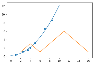
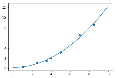
最小二乘法求解函数 scipy.linalg.lstsq,现在用其完成一个最小二乘求解过程
首先给出样本的 (x) 和 (y) 值。然后假设其符合 (y = ax^2 + b) 分布
import numpy as np
x = np.array([1, 2.5, 3.5, 4, 5, 7, 8.5])
y = np.array([0.3, 1.1, 1.5, 2.0, 3.2, 6.6, 8.6])
然后计算 (x^2) ,并添加截距项系数 1
M = x[:, np.newaxis]**[0, 2]
print(M)
#输出 $x^2$
[[  1.     1.  ]
 [  1.     6.25]
 [  1.    12.25]
 ...,
 [  1.    25.  ]
 [  1.    49.  ]
 [  1.    72.25]]
接着使用 linalg.lstsq 执行最小二乘法计算,返回的第一组参数即为拟合系数
from scipy import linalg
p = linalg.lstsq(M, y)[0]
print(p)
#输出拟合系数
[ 0.20925829  0.12013861]
最后,通过绘图查看最小二乘法得到的参数是否合理,绘制样本和拟合曲线图。
from matplotlib import pyplot as plt
plt.scatter(x, y)
xx = np.linspace(0, 10, 100)
yy = p[0] + p[1]*xx**2
plt.plot(xx, yy)
- 插值函数
插值是数值分析领域中通过已知的、离散的数据点,在范围内推求新数据点的过程或方法。SciPy 提供的 scipy.interpolate 模块包含了大量的数学插值方法。
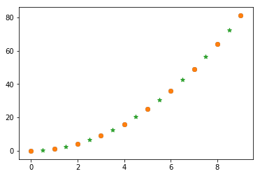
例如,使用 SciPy 完成线性插值的过程。首先,给出一组 (x) 和 (y) 的值。
import numpy as np
from matplotlib import pyplot as plt
x = np.array([0, 1, 2, 3, 4, 5, 6, 7, 8, 9])
y = np.array([0, 1, 4, 9, 16, 25, 36, 49, 64, 81])
plt.scatter(x, y)

在上方两个点与点之间再插入一个值,这里就可以用到线性插值的方法。
from scipy import interpolate
xx = np.array([0.5, 1.5, 2.5, 3.5, 4.5, 5.5, 6.5, 7.5, 8.5])  #两点之间的点的x坐标
f = interpolate.interp1d(x, y)  #使用原样本点建立插值函数
yy = f(xx)  #映射到新样本点
plt.scatter(x, y)
plt.scatter(xx, yy, marker='*')
(5) scikit-learn
scikit-learn简称sklearn,是机器学习的一个开源框架、也是一个重要的Python模块,其中包含多种成熟的算法,包括:
- 分类
- 回归
- 聚类(非监督分类)
- 数据降维
- 模型选择
- 数据预处理
关于scikit-learn的使用方法,可以查看我的另一篇博文Python机器学习(Sebastian著 ) 学习笔记——第六章模型评估与参数调优实战(Windows Spyder Python 3.6)
欢迎大家提供宝贵建议
博客以学习、分享为主!