Tensorflow学习笔记

目录

• tf
  • tf.constant
  • Variable
  • reduce_sum()
  • reduce_mean()
  • tf.ones_like
  • tf.multiply（）
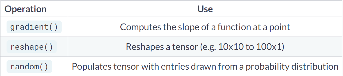
  • tf.gradients
  • tf.reshape
  • path
  • Setting the data type
    • tf.cast()
    • tf.array()
  • loss function
    • mse
    • mae
    • huber
  • Linear regression
    • Multiple linear regression
  • Batch training
    • chunksize
  • Dense layers
    • 自定义dense层
  • Activation functions
  • Multiclass classification problems
  • Optimizers
  • 随机初始化权重矩阵和bias
  • 创建函数定义模型和损失函数
    • 梯度下降进行优化
  • Defining neural networks with Keras
    • sequence
    • compile
  • Defining a multiple input model
  • Training and validation with Keras
  • validation
  • Overfitting detection
  • Evaluate
  • Training models with the Estimators API
    • 定义特征变量
  • 完成证书

tf

tf.constant

创建一个常量
tf.constant(value,dtype=None,shape=None,name=’Const’)
创建一个常量tensor，按照给出value来赋值，可以用shape来指定其形状。value可以是一个数，也可以是一个list。
如果是一个数，那么这个常量中所有值的按该数来赋值。
如果是list,那么len(value)一定要小于等于shape展开后的长度。赋值时，先将value中的值逐个存入。不够的部分，则全部存入value的最后一个值。

Variable

创建变量

reduce_sum()

压缩求和，用于降维（可以指定按照行或者列）

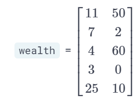
按列求和

 reduce_sum(wealth,1).numpy()
Out[4]: array([61,  9, 64,  3, 35], dtype=int32)

reduce_mean()

求平均
reduce_max()
求最大值

tf.ones_like

tf.ones_like(tensor,dype=None,name=None)
tf.zeros_like(tensor,dype=None,name=None)
新建一个与给定的tensor类型大小一致的tensor，其所有元素为1和0

tf.multiply（）

算两个tensor的乘积，对应位置相乘

两个矩阵中对应元素各自相乘
格式: tf.multiply(x, y, name=None)
参数:
x: 一个类型为:half, float32, float64, uint8, int8, uint16, int16, int32, int64, complex64, complex128的张量。
y: 一个类型跟张量x相同的张量。
返回值： x * y element-wise.
注意：
（1）multiply这个函数实现的是元素级别的相乘，也就是两个相乘的数元素各自相乘，而不是矩阵乘法，注意和tf.matmul区别。
（2）两个相乘的数必须有相同的数据类型，不然就会报错。

2.tf.matmul（）将矩阵a乘以矩阵b，生成a * b。
格式: tf.matmul(a, b, transpose_a=False, transpose_b=False, adjoint_a=False, adjoint_b=False, a_is_sparse=False, b_is_sparse=False, name=None)
参数:
a: 一个类型为 float16, float32, float64, int32, complex64, complex128 且张量秩 > 1 的张量。
b: 一个类型跟张量a相同的张量。
transpose_a: 如果为真, a则在进行乘法计算前进行转置。
transpose_b: 如果为真, b则在进行乘法计算前进行转置。
adjoint_a: 如果为真, a则在进行乘法计算前进行共轭和转置。
adjoint_b: 如果为真, b则在进行乘法计算前进行共轭和转置。
a_is_sparse: 如果为真, a会被处理为稀疏矩阵。
b_is_sparse: 如果为真, b会被处理为稀疏矩阵。
name: 操作的名字（可选参数）
返回值： 一个跟张量a和张量b类型一样的张量且最内部矩阵是a和b中的相应矩阵的乘积。
注意：
（1）输入必须是矩阵（或者是张量秩 >２的张量，表示成批的矩阵），并且其在转置之后有相匹配的矩阵尺寸。
（2）两个矩阵必须都是同样的类型，支持的类型如下：float16, float32, float64, int32, complex64, complex128。
引发错误:
ValueError: 如果transpose_a 和 adjoint_a, 或 transpose_b 和 adjoint_b 都被设置为真

In [1]: features = constant([[2, 24], [2, 26], [2, 57], [1, 37]])
... params = constant([[1000], [150]])

In [2]: billpred = matmul(features, params)

In [3]: billpred
Out[3]: 
<tf.Tensor: shape=(4, 1), dtype=int32, numpy=
array([[ 5600],
       [ 5900],
       [10550],
       [ 6550]], dtype=int32)>

注意这个矩阵的形式：
features = constant([[2, 24], [2, 26], [2, 57], [1, 37]])
表现出来应该是这个，别把矩阵的形式搞混。

2 24
2 26 
2 57
1 37

tf.gradients

用来进行梯度求解

def compute_gradient(x0):
  	# Define x as a variable with an initial value of x0
	x = Variable(x0)
	with GradientTape() as tape:
		tape.watch(x)
        # Define y using the multiply operation
		y = multiply(x, x)
    # Return the gradient of y with respect to x
	return tape.gradient(y, x).numpy()

# Compute and print gradients at x = -1, 1, and 0
print(compute_gradient(-1.0))
print(compute_gradient(1.0))
print(compute_gradient(0.0))

<script.py> output:
    -2.0
    2.0
    0.0

tf.reshape

重新指定张量的维度

# Reshape the grayscale image tensor into a vector
gray_vector = reshape(gray_tensor, (784, 1))

# Reshape model from a 1x3 to a 3x1 tensor
model = reshape(model, (3, 1))

# Multiply letter by model
output = matmul(letter, model)

# Sum over output and print prediction using the numpy method，这里的输出为啥要降维还没太懂
prediction = reduce_sum(output)
# 这里要记得把输出变成一个numpy数组，不然输出会报错
print(prediction.numpy())

path

路径单独写出来可以批量导入，或者导出，这是一个既定的规则

# Import pandas under the alias pd
import pandas as pd

# Assign the path to a string variable named data_path
data_path = 'kc_house_data.csv'

# Load the dataset as a dataframe named housing
housing = pd.read_csv(data_path)

# Print the price column of housing
print(housing['price'])

Setting the data type

tf.cast()

函数的作用是执行 tensorflow 中张量数据类型转换

tf.array()

# Import numpy and tensorflow with their standard aliases
import numpy as np
import tensorflow as tf


# Use a numpy array to define price as a 32-bit float
price = np.array(housing['price'], np.float)

# Define waterfront as a Boolean using cast
waterfront = tf.cast(housing['waterfront'], tf.bool)

# Print price and waterfront
print(price)
print(waterfront)

<script.py> output:
    [221900. 538000. 180000. ... 402101. 400000. 325000.]
    tf.Tensor([False False False ... False False False], shape=(21613,), dtype=bool)

loss function

mse

均值误差

mae

平均绝对值误差

# Import the keras module from tensorflow
from tensorflow import keras

# Compute the mean absolute error (mae)
loss = keras.losses.mse(price, predictions)
loss = keras.losses.mae(price, predictions)
# Print the mean absolute error (mae)
print(loss.numpy())

<script.py> output:
    141171604777.12717

<script.py> output:
    268827.99302087986

# Initialize a variable named scalar
scalar = Variable(1.0, float32)

# Define the model
def model(scalar, features = features):
  	return scalar * features

# Define a loss function
def loss_function(scalar, features = features, targets = targets):
	# Compute the predicted values
	predictions = model(scalar, features)
    
	# Return the mean absolute error loss
	return keras.losses.mae(targets, predictions)

# Evaluate the loss function and print the loss
print(loss_function(scalar).numpy())

huber

Linear regression

线性回归

# Define a linear regression model
def linear_regression(intercept, slope, features = size_log):
	return intercept + features*slope

# Set loss_function() to take the variables as arguments
def loss_function(intercept, slope, features = size_log, targets = price_log):
	# Set the predicted values
	predictions = linear_regression(intercept, slope, features)
    
    # Return the mean squared error loss
	return keras.losses.mse(targets, predictions)

# Compute the loss for different slope and intercept values
print(loss_function(0.1, 0.1).numpy())
print(loss_function(0.1, 0.5).numpy())

## 优化器优化,这个是梯度下降优化嘛，我还不太明白

# Initialize an adam optimizer
opt = keras.optimizers.Adam(0.5)

for j in range(100):
	# Apply minimize, pass the loss function, and supply the variables
	opt.minimize(lambda: loss_function(intercept, slope), var_list=[intercept, slope])

	# Print every 10th value of the loss
	if j % 10 == 0:
		print(loss_function(intercept, slope).numpy())

# Plot data and regression line
plot_results(intercept, slope)

Multiple linear regression

其实目前很清晰，就是把数学公式复现，

# Define the linear regression model
def linear_regression(params, feature1 = size_log, feature2 = bedrooms):
	return params[0] + feature1*params[1] + feature2*params[2]

# Define the loss function
def loss_function(params, targets = price_log, feature1 = size_log, feature2 = bedrooms):
	# Set the predicted values
	predictions = linear_regression(params, feature1, feature2)
  
	# Use the mean absolute error loss
	return keras.losses.mae(targets, predictions)

# Define the optimize operation
opt = keras.optimizers.Adam()

# Perform minimization and print trainable variables
for j in range(10):
	opt.minimize(lambda: loss_function(params), var_list=[params])
	print_results(params)

Batch training

（1）iteration：表示1次迭代（也叫training step），每次迭代更新1次网络结构的参数；
（2）batch-size：1次迭代所使用的样本量；
（3）epoch：1个epoch表示过了1遍训练集中的所有样本。诸葛村姑

chunksize

read_csv中有个参数chunksize，通过指定一个chunksize分块大小来读取文件，返回的是一个可迭代的对象TextFileReader

分块读取大文件，这里分成100块

# Initialize adam optimizer
opt = keras.optimizers.Adam()

# Load data in batches
for batch in pd.read_csv('kc_house_data.csv', chunksize=100):
	size_batch = np.array(batch['sqft_lot'], np.float32)

	# Extract the price values for the current batch
	price_batch = np.array(batch['price'], np.float32)

	# Complete the loss, fill in the variable list, and minimize
	opt.minimize(lambda: loss_function(intercept, slope, price_batch, size_batch), var_list=[intercept, slope])

# Print trained parameters
print(intercept.numpy(), slope.numpy())

Dense layers

yi'zhi

一直没太搞明白dense层到底是哪个层。。
这个图的话给了很好的解释，就是hiden layer

这样简单定义一个网络结构就比较清晰了

# From previous step
bias1 = Variable(1.0)
weights1 = Variable(ones((3, 2)))
product1 = matmul(borrower_features, weights1)
dense1 = keras.activations.sigmoid(product1 + bias1)

# Initialize bias2 and weights2
bias2 = Variable(1.0)
weights2 = Variable(ones((2, 1)))

# Perform matrix multiplication of dense1 and weights2
product2 = matmul(dense1 ,weights2)

# Apply activation to product2 + bias2 and print the prediction
prediction = keras.activations.sigmoid(product2 + bias2)
print('
 prediction: {}'.format(prediction.numpy()[0,0]))
print('
 actual: 1')

神经网络是一个看上去很阔怕，但是很底层原理很简答的东西，就是很多线性运算和矩阵相乘
比如这个栗子

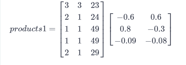
    # Compute the product of borrower_features and weights1
products1 = matmul(borrower_features, weights1)

# Apply a sigmoid activation function to products1 + bias1
dense1 = keras.activations.sigmoid(products1 + bias1)

# Print the shapes of borrower_features, weights1, bias1, and dense1
print('
 shape of borrower_features: ', borrower_features.shape)
print('
 shape of weights1: ', weights1.shape)
print('
 shape of bias1: ', bias1.shape)
print('
 shape of dense1: ', dense1.shape)

<script.py> output:
    
     shape of borrower_features:  (5, 3)
    
     shape of weights1:  (3, 2)
    
     shape of bias1:  (1,)
    
     shape of dense1:  (5, 2)

自定义dense层

keras.layers.Dense(units, 
activation=None, 
use_bias=True, 
kernel_initializer='glorot_uniform', 
bias_initializer='zeros', 
kernel_regularizer=None, 
bias_regularizer=None, 
activity_regularizer=None, 
kernel_constraint=None, 
bias_constraint=None)
				      

# 参数说明
units:
该层有几个神经元

activation:
该层使用的激活函数

use_bias:
是否添加偏置项

kernel_initializer:
权重初始化方法

bias_initializer:
偏置值初始化方法

kernel_regularizer:
权重规范化函数

bias_regularizer:
偏置值规范化方法

activity_regularizer:
输出的规范化方法

kernel_constraint:
权重变化限制函数

bias_constraint:
偏置值变化限制函数

这个栗子里面的话就是有2个hiden layer

# Define the first dense layer
dense1 = keras.layers.Dense(7, activation='sigmoid')(borrower_features)

# Define a dense layer with 3 output nodes
dense2 = keras.layers.Dense(3, activation='sigmoid')(dense1)

# Define a dense layer with 1 output node
predictions = keras.layers.Dense(1, activation='sigmoid')(dense2)

# Print the shapes of dense1, dense2, and predictions
print('
 shape of dense1: ', dense1.shape)
print('
 shape of dense2: ', dense2.shape)
print('
 shape of predictions: ', predictions.shape)

<script.py> output:
    
     shape of dense1:  (100, 7)
    
     shape of dense2:  (100, 3)
    
     shape of predictions:  (100, 1)

Activation functions

Define inputs as a 32-bit floating point constant tensor using bill_amounts.
Set dense1 to be a dense layer with 3 output nodes and a relu activation function.
Set dense2 to be a dense layer with 2 output nodes and a relu activation function.
Set the output layer to be a dense layer with a single output node and a sigmoid activation function.
# 目前觉得这样的写法很清晰，似乎可以得到每一层想要的东西，比keras的另一种写法要好很多
# Construct input layer from features
inputs = constant(bill_amounts, float32)
# dense层的第一个参数指定输出结点数
# Define first dense layer
dense1 = keras.layers.Dense(3, activation='relu')(inputs)

# Define second dense layer
dense2 = keras.layers.Dense(2, activation='relu')(dense1)

# Define output layer
outputs = keras.layers.Dense(1, activation='sigmoid')(dense2)

# Print error for first five examples
error = default[:5] - outputs.numpy()[:5]
print(error)

<script.py> output:
    [[ 1. ]
     [ 1. ]
     [ 0. ]
     [ 0. ]
     [-0.5]]

Multiclass classification problems

多分类问题
其实就是output层的units变成>1的数

# Construct input layer from borrower features
inputs = constant(borrower_features, float32)

# Define first dense layer
dense1 = keras.layers.Dense(10, activation='sigmoid')(inputs)

# Define second dense layer
dense2 = keras.layers.Dense(8, activation='relu')(dense1)

# Define output layer
outputs = keras.layers.Dense(6, activation='softmax')(dense2)

# Print first five predictions
print(outputs.numpy()[:5])

<script.py> output:
    [[0.11626432 0.1127151  0.25804487 0.24624525 0.15216675 0.11456368]
     [0.22433662 0.0683961  0.28301975 0.260067   0.07099433 0.09318623]
     [0.17588586 0.12475339 0.13749284 0.2883481  0.11527162 0.15824823]
     [0.09378582 0.14427742 0.20788462 0.21056697 0.2047638  0.13872144]
     [0.14584291 0.11100206 0.27645484 0.21310686 0.13811046 0.1154829 ]]

Optimizers

优化器
一般会把model定义为一个函数
把loss function定义为一个函数

# Initialize x_1 and x_2
x_1 = Variable(6.0,float32)
x_2 = Variable(0.3,float32)

# Define the optimization operation
opt = keras.optimizers.SGD(learning_rate=0.01)

for j in range(100):
	# Perform minimization using the loss function and x_1
	opt.minimize(lambda: loss_function(x_1), var_list=[x_1])
	# Perform minimization using the loss function and x_2
	opt.minimize(lambda: loss_function(x_2), var_list=[x_2])

# Print x_1 and x_2 as numpy arrays
print(x_1.numpy(), x_2.numpy())

换个损失函数

# Initialize x_1 and x_2
x_1 = Variable(0.05,float32)
x_2 = Variable(0.05,float32)

# Define the optimization operation for opt_1 and opt_2
opt_1 = keras.optimizers.RMSprop(learning_rate=0.01, momentum=0.99)
opt_2 = keras.optimizers.RMSprop(learning_rate=0.01, momentum=0.00)

## 这里就是迭代100次的损失函数
for j in range(100):
	opt_1.minimize(lambda: loss_function(x_1), var_list=[x_1])
    # Define the minimization operation for opt_2
	opt_2.minimize(lambda: loss_function(x_2), var_list=[x_2])

# Print x_1 and x_2 as numpy arrays
print(x_1.numpy(), x_2.numpy())

随机初始化权重矩阵和bias

# Define the layer 1 weights
w1 = Variable(random.normal([23, 7]))

# Initialize the layer 1 bias
b1 = Variable(ones([7]))

# Define the layer 2 weights
w2 = Variable(random.normal([7, 1]))

# Define the layer 2 bias
b2 = Variable(0.0)

创建函数定义模型和损失函数

# Define the model
def model(w1, b1, w2, b2, features = borrower_features):
	# Apply relu activation functions to layer 1
	layer1 = keras.activations.relu(matmul(features, w1) + b1)
    # Apply dropout
	dropout = keras.layers.Dropout(0.25)(layer1)
	return keras.activations.sigmoid(matmul(dropout, w2) + b2)

# Define the loss function
def loss_function(w1, b1, w2, b2, features = borrower_features, targets = default):
	predictions = model(w1, b1, w2, b2)
	# Pass targets and predictions to the cross entropy loss
	return keras.losses.binary_crossentropy(targets, predictions)

梯度下降进行优化

# Train the model
# 迭代100次
for j in range(100):
    # Complete the optimizer
	opt.minimize(lambda: loss_function(w1, b1, w2, b2), 
                 var_list=[w1, b1, w2, b2])

# Make predictions with model
model_predictions = model(w1, b1, w2, b2,test_features)

# Construct the confusion matrix，看来混淆矩阵可以输出
confusion_matrix(test_targets, model_predictions)

Defining neural networks with Keras

其实就是序列化的输入方式

sequence

其实这里想想真的很方便，定义
输入层input
隐藏层hiden layer （可以以一层，可以多层，按照顺序拼接就好）
输出层output
然后按照顺序拼接起来

使用keras是有两种方式的，一种是直接定义好一个sequential，然后一直add层就好了

# Define a Keras sequential model
model = keras.Sequential()

# Define the first dense layer
model.add(keras.layers.Dense(16, activation='relu', input_shape=(784,)))

# Define the second dense layer
model.add(keras.layers.Dense(8, activation='relu'))

# Define the output layer
model.add(keras.layers.Dense(4, activation='softmax'))

# Print the model architecture
print(model.summary())

<script.py> output:
    Model: "sequential"
    _________________________________________________________________
    Layer (type)                 Output Shape              Param #   
    =================================================================
    dense (Dense)                (None, 16)                12560     
    _________________________________________________________________
    dense_1 (Dense)              (None, 8)                 136       
    _________________________________________________________________
    dense_2 (Dense)              (None, 4)                 36        
    =================================================================
    Total params: 12,732
    Trainable params: 12,732
    Non-trainable params: 0
    _________________________________________________________________
    None

定义好一个sequence之后编译complie

compile

# Define the first dense layer
model.add(keras.layers.Dense(16, activation='sigmoid', input_shape=(784,)))

# Apply dropout to the first layer's output
model.add(keras.layers.Dropout(0.25))

# Define the output layer
model.add(keras.layers.Dense(4, activation='softmax'))

# Compile the model
model.compile('adam', loss='categorical_crossentropy')

# Print a model summary
print(model.summary())

<script.py> output:
    Model: "sequential"
    _________________________________________________________________
    Layer (type)                 Output Shape              Param #   
    =================================================================
    dense (Dense)                (None, 16)                12560     
    _________________________________________________________________
    dropout (Dropout)            (None, 16)                0         
    _________________________________________________________________
    dense_1 (Dense)              (None, 4)                 68        
    =================================================================
    Total params: 12,628
    Trainable params: 12,628
    Non-trainable params: 0
    _________________________________________________________________
    None

Defining a multiple input model

定义一个多输入的网络模型
多输入和多输出

# For model 1, pass the input layer to layer 1 and layer 1 to layer 2
m1_layer1 = keras.layers.Dense(12, activation='sigmoid')(m1_inputs)
m1_layer2 = keras.layers.Dense(4, activation='softmax')(m1_layer1)

# For model 2, pass the input layer to layer 1 and layer 1 to layer 2
m2_layer1 = keras.layers.Dense(12, activation='relu')(m2_inputs)
m2_layer2 = keras.layers.Dense(4, activation='softmax')(m2_layer1)

# Merge model outputs and define a functional model
merged = keras.layers.add([m1_layer2, m2_layer2])
model = keras.Model(inputs=[m1_inputs, m2_inputs], outputs=merged)

# Print a model summary
print(model.summary())

<script.py> output:
    Model: "model"
    __________________________________________________________________________________________________
    Layer (type)                    Output Shape         Param #     Connected to                     
    ==================================================================================================
    input_1 (InputLayer)            [(None, 784)]        0                                            
    __________________________________________________________________________________________________
    input_2 (InputLayer)            [(None, 784)]        0                                            
    __________________________________________________________________________________________________
    dense (Dense)                   (None, 12)           9420        input_1[0][0]                    
    __________________________________________________________________________________________________
    dense_2 (Dense)                 (None, 12)           9420        input_2[0][0]                    
    __________________________________________________________________________________________________
    dense_1 (Dense)                 (None, 4)            52          dense[0][0]                      
    __________________________________________________________________________________________________
    dense_3 (Dense)                 (None, 4)            52          dense_2[0][0]                    
    __________________________________________________________________________________________________
    add (Add)                       (None, 4)            0           dense_1[0][0]                    
                                                                     dense_3[0][0]                    
    ==================================================================================================
    Total params: 18,944
    Trainable params: 18,944
    Non-trainable params: 0
    __________________________________________________________________________________________________
    None

Training and validation with Keras

# Define a sequential model
model = keras.Sequential()

# Define a hidden layer
model.add(keras.layers.Dense(16, activation='relu', input_shape=(784,)))

# Define the output layer
model.add(keras.layers.Dense(4, activation='softmax'))

# Compile the model
model.compile('SGD', loss='categorical_crossentropy')

# Complete the fitting operation
model.fit(sign_language_features, sign_language_labels, epochs=5)

<script.py> output:
    Train on 2000 samples
    Epoch 1/5
    
  32/2000 [..............................] - ETA: 30s - loss: 1.5861
 640/2000 [========>.....................] - ETA: 1s - loss: 1.3109 
1280/2000 [==================>...........] - ETA: 0s - loss: 1.2190
1920/2000 [===========================>..] - ETA: 0s - loss: 1.1552
2000/2000 [==============================] - 1s 328us/sample - loss: 1.1465
    Epoch 2/5
    
  32/2000 [..............................] - ETA: 0s - loss: 0.9728
 672/2000 [=========>....................] - ETA: 0s - loss: 0.9270
1312/2000 [==================>...........] - ETA: 0s - loss: 0.8795
1952/2000 [============================>.] - ETA: 0s - loss: 0.8326
2000/2000 [==============================] - 0s 81us/sample - loss: 0.8299
    Epoch 3/5
    
  32/2000 [..............................] - ETA: 0s - loss: 0.5687
 672/2000 [=========>....................] - ETA: 0s - loss: 0.6832
1312/2000 [==================>...........] - ETA: 0s - loss: 0.6657
1952/2000 [============================>.] - ETA: 0s - loss: 0.6453
2000/2000 [==============================] - 0s 81us/sample - loss: 0.6441
    Epoch 4/5
    
  32/2000 [..............................] - ETA: 0s - loss: 0.5858
 672/2000 [=========>....................] - ETA: 0s - loss: 0.5500
1312/2000 [==================>...........] - ETA: 0s - loss: 0.5479
1952/2000 [============================>.] - ETA: 0s - loss: 0.5322
2000/2000 [==============================] - 0s 80us/sample - loss: 0.5300
    Epoch 5/5
    
  32/2000 [..............................] - ETA: 0s - loss: 0.3786
 672/2000 [=========>....................] - ETA: 0s - loss: 0.4668
1312/2000 [==================>...........] - ETA: 0s - loss: 0.4582
1952/2000 [============================>.] - ETA: 0s - loss: 0.4504
2000/2000 [==============================] - 0s 80us/sample - loss: 0.4510

validation

# Define sequential model
model = keras.Sequential()

# Define the first layer
model.add(keras.layers.Dense(32, activation='sigmoid', input_shape=(784,)))

# Add activation function to classifier
model.add(keras.layers.Dense(4, activation='softmax'))

# Set the optimizer, loss function, and metrics
model.compile(optimizer='RMSprop', loss='categorical_crossentropy', metrics=['accuracy'])

# Add the number of epochs and the validation split
model.fit(sign_language_features, sign_language_labels, epochs=10, validation_split=0.1)

<script.py> output:
    Train on 1799 samples, validate on 200 samples
    Epoch 1/10
    
  32/1799 [..............................] - ETA: 43s - loss: 1.4871 - accuracy: 0.2188
 608/1799 [=========>....................] - ETA: 1s - loss: 1.2876 - accuracy: 0.4309 
1216/1799 [===================>..........] - ETA: 0s - loss: 1.1833 - accuracy: 0.5255
1792/1799 [============================>.] - ETA: 0s - loss: 1.1138 - accuracy: 0.5725
1799/1799 [==============================] - 1s 619us/sample - loss: 1.1135 - accuracy: 0.5725 - val_loss: 0.9707 - val_accuracy: 0.5600
    Epoch 2/10
    
  32/1799 [..............................] - ETA: 0s - loss: 0.9954 - accuracy: 0.6250
 608/1799 [=========>....................] - ETA: 0s - loss: 0.8494 - accuracy: 0.7796
1216/1799 [===================>..........] - ETA: 0s - loss: 0.8153 - accuracy: 0.7796
1799/1799 [==============================] - 0s 101us/sample - loss: 0.7811 - accuracy: 0.7916 - val_loss: 0.6716 - val_accuracy: 0.9200
    Epoch 3/10
    
  32/1799 [..............................] - ETA: 0s - loss: 0.6939 - accuracy: 0.8750
 640/1799 [=========>....................] - ETA: 0s - loss: 0.6641 - accuracy: 0.8422
1248/1799 [===================>..........] - ETA: 0s - loss: 0.6311 - accuracy: 0.8534
1799/1799 [==============================] - 0s 100us/sample - loss: 0.5984 - accuracy: 0.8694 - val_loss: 0.5287 - val_accuracy: 0.9400
    Epoch 4/10
    
  32/1799 [..............................] - ETA: 0s - loss: 0.5383 - accuracy: 0.8750
 640/1799 [=========>....................] - ETA: 0s - loss: 0.5119 - accuracy: 0.9031
1248/1799 [===================>..........] - ETA: 0s - loss: 0.4884 - accuracy: 0.9087
1799/1799 [==============================] - 0s 100us/sample - loss: 0.4621 - accuracy: 0.9133 - val_loss: 0.4863 - val_accuracy: 0.8450
    Epoch 5/10
    
  32/1799 [..............................] - ETA: 0s - loss: 0.4294 - accuracy: 0.8438
 640/1799 [=========>....................] - ETA: 0s - loss: 0.3951 - accuracy: 0.9375
1248/1799 [===================>..........] - ETA: 0s - loss: 0.3847 - accuracy: 0.9431
1799/1799 [==============================] - 0s 100us/sample - loss: 0.3686 - accuracy: 0.9489 - val_loss: 0.4299 - val_accuracy: 0.9250
    Epoch 6/10
    
  32/1799 [..............................] - ETA: 0s - loss: 0.3646 - accuracy: 0.9375
 640/1799 [=========>....................] - ETA: 0s - loss: 0.3231 - accuracy: 0.9547
1216/1799 [===================>..........] - ETA: 0s - loss: 0.3070 - accuracy: 0.9646
1799/1799 [==============================] - 0s 106us/sample - loss: 0.2930 - accuracy: 0.9672 - val_loss: 0.3686 - val_accuracy: 0.7850
    Epoch 7/10
    
  32/1799 [..............................] - ETA: 0s - loss: 0.2952 - accuracy: 0.8438
 352/1799 [====>.........................] - ETA: 0s - loss: 0.2509 - accuracy: 0.9659
 704/1799 [==========>...................] - ETA: 0s - loss: 0.2546 - accuracy: 0.9659
1056/1799 [================>.............] - ETA: 0s - loss: 0.2447 - accuracy: 0.9697
1312/1799 [====================>.........] - ETA: 0s - loss: 0.2396 - accuracy: 0.9733
1728/1799 [===========================>..] - ETA: 0s - loss: 0.2398 - accuracy: 0.9722
1799/1799 [==============================] - 0s 173us/sample - loss: 0.2415 - accuracy: 0.9711 - val_loss: 0.2143 - val_accuracy: 0.9850
    Epoch 8/10
    
  32/1799 [..............................] - ETA: 0s - loss: 0.2202 - accuracy: 1.0000
 448/1799 [======>.......................] - ETA: 0s - loss: 0.2020 - accuracy: 0.9754
 800/1799 [============>.................] - ETA: 0s - loss: 0.2098 - accuracy: 0.9712
1216/1799 [===================>..........] - ETA: 0s - loss: 0.1987 - accuracy: 0.9753
1664/1799 [==========================>...] - ETA: 0s - loss: 0.1941 - accuracy: 0.9766
1799/1799 [==============================] - 0s 150us/sample - loss: 0.1921 - accuracy: 0.9778 - val_loss: 0.2852 - val_accuracy: 0.8650
    Epoch 9/10
    
  32/1799 [..............................] - ETA: 0s - loss: 0.2495 - accuracy: 0.8438
 480/1799 [=======>......................] - ETA: 0s - loss: 0.1926 - accuracy: 0.9625
 992/1799 [===============>..............] - ETA: 0s - loss: 0.1783 - accuracy: 0.9798
1504/1799 [========================>.....] - ETA: 0s - loss: 0.1654 - accuracy: 0.9827
1799/1799 [==============================] - 0s 121us/sample - loss: 0.1583 - accuracy: 0.9850 - val_loss: 0.2024 - val_accuracy: 0.9500
    Epoch 10/10
    
  32/1799 [..............................] - ETA: 0s - loss: 0.2180 - accuracy: 0.9375
 480/1799 [=======>......................] - ETA: 0s - loss: 0.1492 - accuracy: 0.9729
 992/1799 [===============>..............] - ETA: 0s - loss: 0.1467 - accuracy: 0.9758
1536/1799 [========================>.....] - ETA: 0s - loss: 0.1389 - accuracy: 0.9798
1799/1799 [==============================] - 0s 131us/sample - loss: 0.1360 - accuracy: 0.9822 - val_loss: 0.1397 - val_accuracy: 0.9650

Overfitting detection

过拟合检测

# Define sequential model
model = keras.Sequential()

# Define the first layer
model.add(keras.layers.Dense(1024, activation='relu', input_shape=(784,)))

# Add activation function to classifier
model.add(keras.layers.Dense(4, activation='softmax'))

# Finish the model compilation
model.compile(optimizer=keras.optimizers.Adam(lr=0.01), 
              loss='categorical_crossentropy', metrics=['accuracy'])

# Complete the model fit operation
model.fit(sign_language_features, sign_language_labels, epochs=200, validation_split=0.5)

Evaluate

# Evaluate the small model using the train data
small_train = small_model.evaluate(train_features, train_labels)

# Evaluate the small model using the test data
small_test = small_model.evaluate(test_features, test_labels)

# Evaluate the large model using the train data
large_train = large_model.evaluate(train_features, train_labels)

# Evaluate the large model using the test data
large_test = large_model.evaluate(test_features, test_labels)

# Print losses
print('
 Small - Train: {}, Test: {}'.format(small_train, small_test))
print('Large - Train: {}, Test: {}'.format(large_train, large_test))

Training models with the Estimators API

定义特征变量

# Define feature columns for bedrooms and bathrooms
bedrooms = feature_column.numeric_column("bedrooms")
bathrooms = feature_column.numeric_column("bathrooms")

# Define the list of feature columns
feature_list = [bedrooms, bathrooms]

def input_fn():
	# Define the labels
	labels = np.array(housing['price'])
	# Define the features
	features = {'bedrooms':np.array(housing['bedrooms']), 
                'bathrooms':np.array(housing['bathrooms'])}
	return features, labels

完成证书