隐马尔科夫模型研究 stock 以及 lotto

说明

本文参考了这里

由于数据是连续的，因此使用了高斯隐马尔科夫模型：gaussianHMM

一、stock代码

import tushare as ts
import pandas as pd
import numpy as np
from hmmlearn.hmm import GaussianHMM

from matplotlib import cm, pyplot as plt
import seaborn as sns
sns.set_style('white')

'''
假定隐藏状态数目为4，观测状态数目为2
'''

# 1.准备 X 
df = ts.get_hist_data('sh',start='2014-01-01',end='2017-07-27')[::-1] # 上证指数

close = np.log(df['close'])
low, high = np.log(df['low']), np.log(df['high'])
t = 5
X = pd.concat([close.diff(1), close.diff(t), high-low], axis=1)[t:] # 显状态时间序列（观测得到）


# 2.拟合 HMM
model = GaussianHMM(n_components=6, covariance_type="diag", n_iter=1000).fit(X)
Z = model.predict(X) # 隐状态时间序列


# 3.画图看看
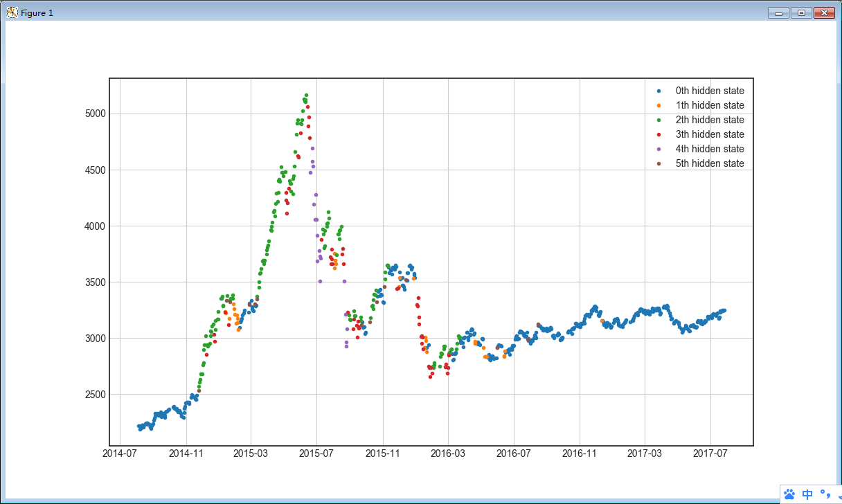
plt.figure(figsize=(12, 7))  
for i in range(model.n_components):
    mask = (Z==i) # 注意这里的Z!!!
    plt.plot_date(df.index[t:][mask], df['close'][t:][mask],'.',label=f'{i}th hidden state',lw=1)
    plt.legend()
    plt.grid(1)

plt.show()

效果图

解释

下面是对6种隐状态的一种可能的解释：【图文对不上，文字来自这里】

• 状态0————蓝色————震荡下跌
• 状态1————绿色————小幅的上涨
• 状态2————红色————牛市上涨
• 状态3————紫色————牛市下跌
• 状态4————黄色————震荡下跌
• 状态5————浅蓝色————牛市下跌
  以上的意义归结是存在一定主观性的。因为HMM模型对输入的多维度观测变量进行处理后，只负责分出几个类别，而并不会定义出每种类别的实际含义。所以我们从图形中做出上述的判断。

所以，这种方法本质上是一种 Classification（分类） 或者 Clustering（聚类）

二、lotto 代码

import tushare as ts
import pandas as pd
import numpy as np
from hmmlearn.hmm import GaussianHMM

from matplotlib import cm, pyplot as plt
from matplotlib.widgets import MultiCursor

import seaborn as sns
sns.set_style('white')

import marksix_1
import talib as ta

'''
假定隐藏状态数目为6，观测状态数目为4
'''

# 1.准备 X 
lt = marksix_1.Marksix()
lt.load_data(period=1000)

#series = lt.adapter(loc='0000001', zb_name='ptsx', args=(1,), tf_n=0)
m = 2
series = lt.adapter(loc='0000001', zb_name='mod', args=(m, lt.get_mod_list(m)), tf_n=0)
# 实时线
close = np.cumsum(series).astype(float)

# 低阶数据
t1, t2, t3 = 5, 10, 20
ma1 = ta.MA(close, timeperiod=t1, matype=0)
std1 = ta.STDDEV(close, timeperiod=t1, nbdev=1)

ma2 = ta.MA(close, timeperiod=t2, matype=0)
std2 = ta.STDDEV(close, timeperiod=t2, nbdev=1)

ma3 = ta.MA(close, timeperiod=t3, matype=0)
std3 = ta.STDDEV(close, timeperiod=t3, nbdev=1)

# 转换一
'''
t = t3
X = pd.DataFrame({'ma1':ma1,'ma2':ma2,'ma3':ma3,'std1':std1,'std2':std2,'std3':std3}, index=lt.df.index)[t:]
'''

# 转换二
t = t2
X = pd.DataFrame({'ma1':ma1,'ma2':ma2,'std1':std1,'std2':std2}, index=lt.df.index)[t:]

#close = np.log(df['close'])
#low, high = np.log(df['low']), np.log(df['high'])
#t = 5
#X = pd.concat([close.diff(1), close.diff(t), high-low], axis=1)[t:] # 显状态时间序列（观测得到）



# 2.拟合 HMM
model = GaussianHMM(n_components=6, covariance_type="diag", n_iter=1000).fit(X)
Z = model.predict(X) # 隐状态时间序列



# 3.画图看看
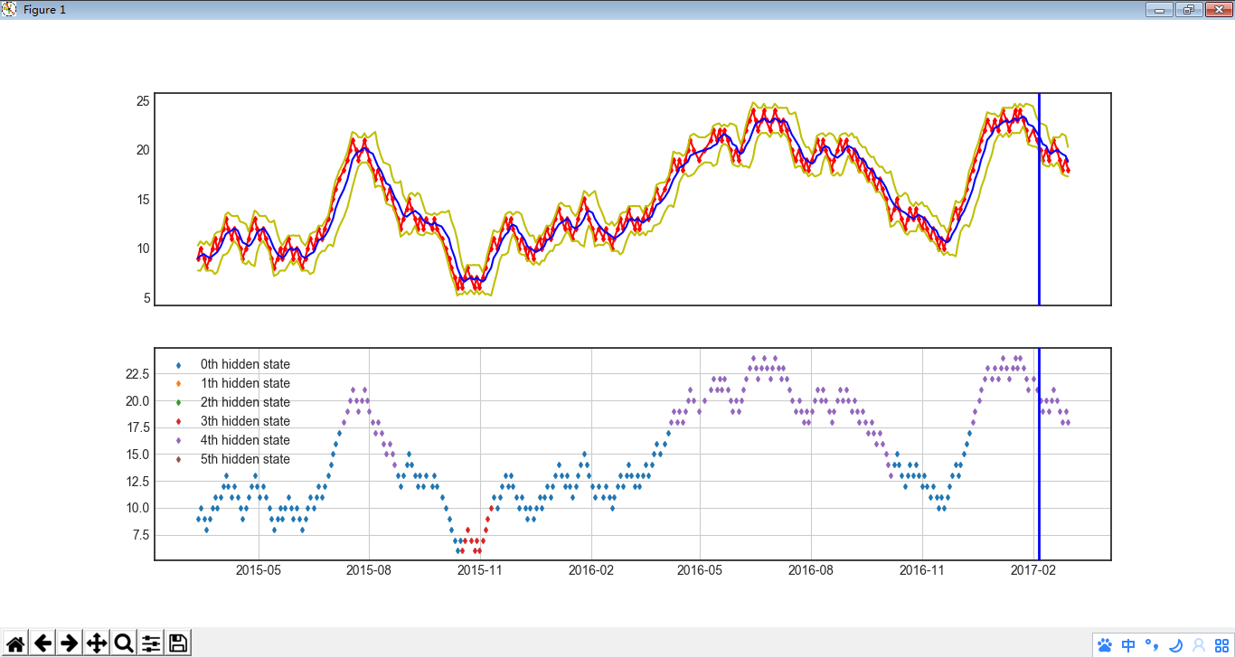
fig, axes = plt.subplots(2, 1, sharex=True)
ax1, ax2 = axes[0], axes[1]

show_period = 300
# 布林线
upperband, middleband, lowerband = ta.BBANDS(close, timeperiod=5, nbdevup=2, nbdevdn=2, matype=0)
axes[0].plot_date(lt.df.index[-show_period:], close[-show_period:], 'rd-', markersize = 3)
axes[0].plot_date(lt.df.index[-show_period:], upperband[-show_period:], 'y-')
axes[0].plot_date(lt.df.index[-show_period:], middleband[-show_period:], 'b-')
axes[0].plot_date(lt.df.index[-show_period:], lowerband[-show_period:], 'y-')

for i in range(model.n_components):
    mask = (Z[-show_period:]==i) # 注意这里的Z!!!
    axes[1].plot_date(lt.df.index[-show_period:][mask], close[-show_period:][mask],'d',markersize=3,label=f'{i}th hidden state',lw=1)
    axes[1].legend()
    axes[1].grid(1)

multi = MultiCursor(fig.canvas, (axes[0], axes[1]), color='b', lw=2)

plt.show()

效果图