Stephen Smith's Blog
All things Sage 300…
The Road to TensorFlow – Part 7: Finally Some Code
Introduction
Well after a long journey through Linux, Python, Python Libraries, the Stock Market, an Introduction to Neural Networks and training Neural Networks we are now ready to look at a complete Python example to predict the stock market.
I placed the full source code listing on my Google Drive here. As described in the previous articles you will need to run this on a Mac or on Linux (could be a virtual image) with Python and TensorFlow installed. You will also need to have the various libraries that are imported at the top of the source file installed or you will get an error when you go to run it. I would suggest getting the source file to play with, Python is very fussy about indentation, so copy/paste from the article may introduce indentation errors caused by the blog formatting.
The Neural Network we are running here is a simple feed forward network with four hidden layers and uses the hyperbolic tangent as the activation function in each case. This is a very simple model so don’t use it to invest with real money. Hopefully this article gives a flavour for how to create and train a Neural Network using TensorFlow. Then in future articles we can discuss the limitation of this model and how to improve it.
Import Libraries
First we import all the various libraries we will be using, note tensorflow and numpy as being particularly important.
# Copyright 2016 Stephen Smith

import time
import math
import os
from datetime import date
from datetime import timedelta
import numpy as np
import matplotlib.pyplot as plt
import tensorflow as tf
import pandas as pd
import pandas_datareader as pdr
from pandas_datareader import data, wb
from six.moves import cPickle as pickle
from yahoo_finance import Share
Get Stock Market Data
Next we get the stock market data. If the file stocks.pickle exists we assume we’ve previously saved this file and use it. Otherwise we get the data from Yahoo Finance using a Web Service call, made via the Pandas DataReader. We only keep the adjusted close column and we fill in any NaN’s with the first value we saw (this really only applies to Visa in this case). The data will all be in a standard Pandas data frame after this.
# Choose amount of historical data to use NHistData
NHistData = 30
TrainDataSetSize = 3000

# Load the Dow 30 stocks from Yahoo into a Pandas datasheet

dow30 = ['AXP', 'AAPL', 'BA', 'CAT', 'CSCO', 'CVX', 'DD', 'XOM',
         'GE', 'GS', 'HD', 'IBM', 'INTC', 'JNJ', 'KO', 'JPM',
         'MCD', 'MMM', 'MRK', 'MSFT', 'NKE', 'PFE', 'PG',
         'TRV', 'UNH', 'UTX', 'VZ', 'V', 'WMT', 'DIS']

num_stocks = len(dow30)

trainData = None
loadNew = False

# If stocks.pickle exists then this contains saved stock data, so use this,
# else use the Pandas DataReader to get the stock data and then pickle it.
stock_filename = 'stocks.pickle'
if os.path.exists(stock_filename):
    try:
        with open(stock_filename, 'rb') as f:
            trainData = pickle.load(f)
    except Exception as e:
      print('Unable to process data from', stock_filename, ':', e)
      raise
    print('%s already present - Skipping requesting/pickling.' % stock_filename)
else:
    # Get the historical data. Make the date range quite a bit bigger than
    # TrainDataSetSize since there are no quotes for weekends and holidays. This
    # ensures we have enough data.

    f = pdr.data.DataReader(dow30, 'yahoo',
        date.today()-timedelta(days=TrainDataSetSize*2+5), date.today())
    cleanData = f.ix['Adj Close']
    trainData = pd.DataFrame(cleanData)
    trainData.fillna(method='backfill', inplace=True)
    loadNew = True
    print('Pickling %s.' % stock_filename)
    try:
        with open(stock_filename, 'wb') as f:
          pickle.dump(trainData, f, pickle.HIGHEST_PROTOCOL)
    except Exception as e:
        print('Unable to save data to', stock_filename, ':', e)
Normalize the Data
We then normalize the data and remember the factor we used so we can de-normalize the results at the end.
# Normalize the data by dividing each price by the first price for a stock.
# This way all the prices start together at 1.
# Remember the normalizing factors so we can go back to real stock prices
# for our final predictions.
factors = np.ndarray(shape=( num_stocks ), dtype=np.float32)
i = 0
for symbol in dow30:
    factors[i] = trainData[symbol][0]
    trainData[symbol] = trainData[symbol]/trainData[symbol][0]
    i = i + 1
Re-arrange the Data for TensorFlow
Now we need to build up our training data, test data and validation data. We need to format this as input arrays for the Neural Network. Looking at this code, I think true Python programmers will accuse me of being a C programmer (which I am), since I do this all with loops. I’m sure a more experience Python programmer could accomplish this quicker with more array operations. This part of the code is quite slow so we pickle it, so if we re-run with the saved stock data, we can also use saved training data.
# Configure how much of the data to use for training, testing and validation.

usableData = len(trainData.index) - NHistData + 1
#numTrainData =  int(0.6 * usableData)
#numValidData =  int(0.2 * usableData
#numTestData = usableData - numTrainData - numValidData - 1
numTrainData = usableData - 1
numValidData = 0
numTestData = 0

train_dataset = np.ndarray(shape=(numTrainData - 1,
    num_stocks * NHistData), dtype=np.float32)
train_labels = np.ndarray(shape=(numTrainData - 1, num_stocks),
    dtype=np.float32)
valid_dataset = np.ndarray(shape=(max(0, numValidData - 1),
    num_stocks * NHistData), dtype=np.float32)
valid_labels = np.ndarray(shape=(max(0, numValidData - 1),
    num_stocks), dtype=np.float32)
test_dataset = np.ndarray(shape=(max(0, numTestData - 1),
    num_stocks * NHistData), dtype=np.float32)
test_labels = np.ndarray(shape=(max(0, numTestData - 1),
    num_stocks), dtype=np.float32)
final_row = np.ndarray(shape=(1, num_stocks * NHistData),
    dtype=np.float32)
final_row_prices = np.ndarray(shape=(1, num_stocks * NHistData),
    dtype=np.float32)

# Build the taining datasets in the correct format with the matching labels.
# So if calculate based on last 30 stock prices then the desired
# result is the 31st. So note that the first 29 data points can't be used.
# Rather than use the stock price, use the pricing deltas.
pickle_file = "traindata.pickle"
if loadNew == True or not os.path.exists(pickle_file):
    for i in range(1, numTrainData):
        for j in range(num_stocks):
            for k in range(NHistData):
                train_dataset[i-1][j * NHistData + k] = (trainData[dow30[j]][i + k]
                    - trainData[dow30[j]][i + k - 1])
            train_labels[i-1][j] = (trainData[dow30[j]][i + NHistData]
                - trainData[dow30[j]][i + NHistData - 1])

    for i in range(1, numValidData):
        for j in range(num_stocks):
            for k in range(NHistData):
                valid_dataset[i-1][j * NHistData + k] = (trainData[dow30[j]][i + k + numTrainData]
                    - trainData[dow30[j]][i + k + numTrainData - 1])
            valid_labels[i-1][j] = (trainData[dow30[j]][i + NHistData + numTrainData]
                - trainData[dow30[j]][i + NHistData + numTrainData - 1])

    for i in range(1, numTestData):
        for j in range(num_stocks):
            for k in range(NHistData):
                test_dataset[i-1][j * NHistData + k] = (trainData[dow30[j]][i + k + numTrainData + numValidData]
                    - trainData[dow30[j]][i + k + numTrainData + numValidData - 1])
            test_labels[i-1][j] = (trainData[dow30[j]][i + NHistData + numTrainData + numValidData]
                - trainData[dow30[j]][i + NHistData + numTrainData + numValidData - 1])

    try:
      f = open(pickle_file, 'wb')
      save = {
        'train_dataset': train_dataset,
        'train_labels': train_labels,
        'valid_dataset': valid_dataset,
        'valid_labels': valid_labels,
        'test_dataset': test_dataset,
        'test_labels': test_labels,
        }
      pickle.dump(save, f, pickle.HIGHEST_PROTOCOL)
      f.close()
    except Exception as e:
      print('Unable to save data to', pickle_file, ':', e)
      raise

else:
    with open(pickle_file, 'rb') as f:
      save = pickle.load(f)
      train_dataset = save['train_dataset']
      train_labels = save['train_labels']
      valid_dataset = save['valid_dataset']
      valid_labels = save['valid_labels']
      test_dataset = save['test_dataset']
      test_labels = save['test_labels']
      del save  # hint to help gc free up memory

for j in range(num_stocks):
    for k in range(NHistData):
            final_row_prices[0][j * NHistData + k] = (trainData[dow30[j]][k + len(trainData.index - NHistData]
            final_row[0][j * NHistData + k] = (trainData[dow30[j]][k + len(trainData.index) - NHistData]
                - trainData[dow30[j]][k + len(trainData.index) - NHistData - 1])

print('Training set', train_dataset.shape, train_labels.shape)
print('Validation set', valid_dataset.shape, valid_labels.shape)
print('Test set', test_dataset.shape, test_labels.shape)
Accuracy
We now setup an accuracy function that is only used to report how we are doing during training. This isn’t used by the training algorithm. It roughly shows what percentage of predictions are within some tolerance.
# This accuracy function is used for reporting progress during training, it isn't actually
# used for training.
def accuracy(predictions, labels):
  err = np.sum( np.isclose(predictions, labels, 0.0, 0.005) ) / (predictions.shape[0] * predictions.shape[1])
  return (100.0 * err)
TensorFlow Variables
We now start setting up TensorFlow by creating our graph and defining our datasets and variables.
batch_size = 4
num_hidden = 16
num_labels = num_stocks

graph = tf.Graph()

# input is 30 days of dow 30 prices normalized to be between 0 and 1.
# output is 30 values for normalized next day price change of dow stocks
# use a 4 level neural network to compute this.

with graph.as_default():

  # Input data.
  tf_train_dataset = tf.placeholder(
    tf.float32, shape=(batch_size, num_stocks * NHistData))
  tf_train_labels = tf.placeholder(tf.float32, shape=(batch_size, num_labels))
  tf_valid_dataset = tf.constant(valid_dataset)
  tf_test_dataset = tf.constant(test_dataset)
  tf_final_dataset = tf.constant(final_row)

  # Variables.
  layer1_weights = tf.Variable(tf.truncated_normal(
      [NHistData * num_stocks, num_hidden], stddev=0.05))
  layer1_biases = tf.Variable(tf.zeros([num_hidden]))
  layer2_weights = tf.Variable(tf.truncated_normal(
      [num_hidden, num_hidden], stddev=0.05))
  layer2_biases = tf.Variable(tf.constant(1.0, shape=[num_hidden]))
  layer3_weights = tf.Variable(tf.truncated_normal(
      [num_hidden, num_hidden], stddev=0.05))
  layer3_biases = tf.Variable(tf.constant(1.0, shape=[num_hidden]))
  layer4_weights = tf.Variable(tf.truncated_normal(
      [num_hidden, num_labels], stddev=0.05))
  layer4_biases = tf.Variable(tf.constant(1.0, shape=[num_labels]))
TensorFlow Model
We now define our Neural Network model. Hyperbolic Tangent is our activation function and rest is matrix algebra as we described in previous articles.
  # Model.
  def model(data):
    hidden = tf.tanh(tf.matmul(data, layer1_weights) + layer1_biases)
    hidden = tf.tanh(tf.matmul(hidden, layer2_weights) + layer2_biases)
    hidden = tf.tanh(tf.matmul(hidden, layer3_weights) + layer3_biases)
    return tf.matmul(hidden, layer4_weights) + layer4_biases
Training Model
Now we setup the training model and the optimizer to use, namely gradient descent. We also define what are the correct answers to compare against.
  # Training computation.
  logits = model(tf_train_dataset)
  loss = tf.nn.l2_loss( tf.sub(logits, tf_train_labels))

  # Optimizer.
  optimizer = tf.train.GradientDescentOptimizer(0.01).minimize(loss)
  # Predictions for the training, validation, and test data.
  train_prediction = logits
  valid_prediction = model(tf_valid_dataset)
  test_prediction = model(tf_test_dataset)
  next_prices = model(tf_final_dataset)
Run the Model
So far we have setup TensorFlow ready to go, but we haven’t calculated anything. This next set of code executes the training run. It will use the data we’ve provided in the configured batch size to train our network while printing out some intermediate information.
num_steps = 2052

with tf.Session(graph=graph) as session:
  tf.initialize_all_variables().run()
  print('Initialized')
  for step in range(num_steps):
    offset = (step * batch_size) % (train_labels.shape[0] - batch_size)
    batch_data = train_dataset[offset:(offset + batch_size), :]
    batch_labels = train_labels[offset:(offset + batch_size), :]
    feed_dict = {tf_train_dataset : batch_data, tf_train_labels : batch_labels}
    _, l, predictions = session.run(
      [optimizer, loss, train_prediction], feed_dict=feed_dict)
    acc = accuracy(predictions, batch_labels)
    if (step % 100 == 0):
      print('Minibatch loss at step %d: %f' % (step, l))
      print('Minibatch accuracy: %.1f%%' % acc)
      if numValidData > 0:
          print('Validation accuracy: %.1f%%' % accuracy(
              valid_prediction.eval(), valid_labels))
  if numTestData > 0:
      print('Test accuracy: %.1f%%' % accuracy(test_prediction.eval(), test_labels))
Make a Prediction
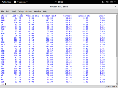
The final bit of code uses our trained model to make a prediction based on the last set of data we have (where we don’t know the right answer). If you get fresh stock market data for today, then the prediction will be for tomorrow’s price changes. If you run this late enough that Yahoo has updated its prices for the day, then you will get some real errors for comparison. Note that Yahoo is very slow and erratic about doing this, so be careful when reading this table.
predictions = next_prices.eval() * factors
  print("Stock    Last Close  Predict Chg   Predict Next      Current     Current Chg       Error")
  i = 0
  for x in dow30:
      yhfeed = Share(x)
      currentPrice = float(yhfeed.get_price())
      print( "%-6s  %9.2f  %9.2f       %9.2f       %9.2f     %9.2f     %9.2f" % (x,
             final_row_prices[0][i * NHistData + NHistData - 1] * factors[i],
             predictions[0][i],
             final_row_prices[0][i * NHistData + NHistData - 1] * factors[i] + predictions[0][i],
             currentPrice,
             currentPrice - final_row_prices[0][i * NHistData + NHistData - 1] * factors[i],
             abs(predictions[0][i] - (currentPrice - final_row_prices[0][i * NHistData + NHistData - 1] * factors[i]))) )
      i = i + 1
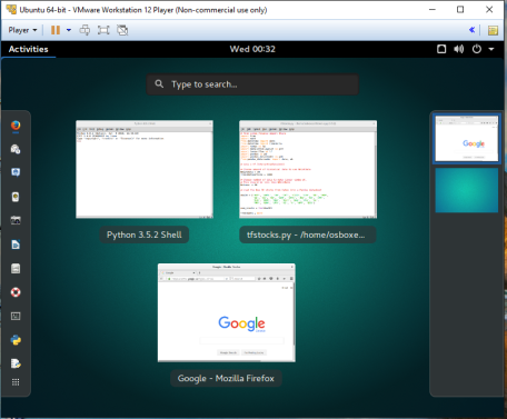
Results
Below is a screenshot of one run predicting the stock changes for Sept. 22. Basically it didn’t do very well. We’ll talk about why and what to do about this in a future article. As you can see it is very conservative in its predictions.
Summary
This article shows the code for training and executing a very simple Neural Network using TensorFlow. Definitely don’t bet on the stock market based on this model, it is very simple at this point. We still need to add a number of elements to start making this into a useful model which we’ll look at in future articles.
The Road to TensorFlow – Part 6: Optimization and Training
Introduction
Last time we looked at the matrix equation that would be our Neural Network which is:
Output of Layer = ActivationFunction( A x (Input of Layer) + b )
We also specified that our input vector would be 900 elements large (the 30 Dow stocks times the last 30 price changes) and the output vector would be 30 elements (then next price change for each of the Dow 30 stocks). This means that if we have just one hidden layer of say 100 Neurons then we need a 900×100 matrix and a 100×30 matrix plus a 100 element bias vector and a 30 element bias vector. This means we need 900×100 + 100×30 + 100 + 30 = 93,130 values. Where do these all come from? In this article we’ll look at where we get these.
Training
What we want to do is use some sort of known or historical data to train the Neural Network. When Neural Networks were first proposed, Computer Scientists tuned these by hand which resulted in taking a long time to get a very small Neural Network that didn’t work well. Later on many methods were developed to calculate these from databases of known cases, however until recently these databases were too small to be effective and led to extreme over-fitting. With the advent of big data, shared cloud resources and automated data collection, a large number of high quality extremely large databases are available to train Neural Networks for well know problems like hand writing recognition or shape identification. Notice that in the introduction to find 93,130 values requires far more than 93,130 bits of data, since this will lead to over-fitting (which we’ll talk a lot about in a future article).
If you remember back to basic statistics and linear regression, we found the best fit for a straight line through a number of data points by minimizing the squares of the distance from the line to each data point. This is why its often called least squares regression. Basically we are formulating the problem as an optimization problem where we are trying to minimize an error function. The linear regression problem is then easily solvable by first year linear algebra. For the Neural Network case it’s a little bit more complicated, but the basic idea is the same.
To train our Neural Network we will use historical data where we provide 30 days of price changes for the Dow 30 stocks and then we know the next change so we can provide the error for our error function. To define an error function, we are going to start by just using the square of the difference, so basically just doing least square minimization just like least squares regression. In TensorFlow we can define our loss function as:
loss = tf.nn.l2_loss( tf.sub(logits, tf_train_labels))
Now that we have the data and an error function how do we go about training our network. First we start by seeding the matrix weights with normally distributed random numbers. TensorFlow provides some help here
layer1_weights = tf.Variable(tf.truncated_normal(
[NHistData * num_stocks, num_hidden], stddev=0.05))
to define our matrix and initialize it with normalized random numbers.
There are a number of optimization algorithms that can be used to solve this problem. The one we are going to use is called Gradient Descent which is a form of Back Propagation. The key property of back propagation algorithms is that they can be applied to Neural Networks with multiple hidden layers. The basic idea is that you take the partial derivative of the loss function with respect to each weight. This gives you a gradient with respect to each weight and then based on whether the gradient is positive or negative you can increase or decrease the weight by a little bit. This little bit is the learning rate which is a parameter to the algorithm (or can be changed dynamically by another algorithm). You then run the training data through this algorithm and hopefully observe your error function decreasing as you go.
This is then the basis of training your network. Once you have the weights you can calculate all the values as you like.
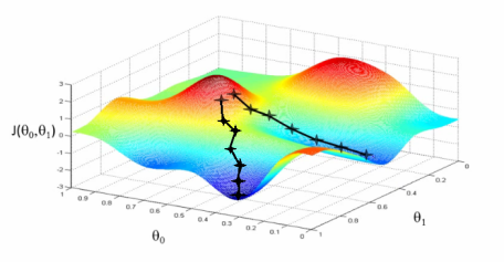
Example of Gradient Descent where it could lead to 2 different minimums
Testing
A big danger here is that you are overfitting. You reduce the error function to next than nothing and the network works well for all your training data. You then try it on something else and it produces very bad results. This is similar to fitting a 10th degree polynomial through 11 data points. It fits all those points exactly, but has no predictive value outside of those exact points.
A common technique is to divide the training data into three buckets: actual training data, testing data and final validation data. You use the training data to train and as you train, you use the testing data to see how you are doing. Then when everything is finished you use the final validation data to do a final test (where the training process has never seen this data). This then gives you an idea of how well the network will fare out in the real world. We will make the size of these three buckets configurable.
Local Versus Global Minimums
During the training process a few different things could happen. The solution could diverge, the error could just keep getting larger and larger. The solution could get stuck in a valley and just orbit a minimum value without converging to it. The solution could converge, but to a local minimum rather than the global minimum. These are all things that need to be watched out for.
Since the initial values are random, re-running the training can lead to quite different solutions. For some problems you want to train repeatedly to get the best solution. Or perhaps compare different optimization algorithms to see which gives the best result. Another idea is to use a combination of algorithms, perhaps start with one that gets into the correct neighborhood, and then another that can zero in on it.
There are quite a few tricks to get out of local minimums and to escape valleys using various random numbers. One is to change the learning rate to occasionally take a bigger jump. Others are to try some random perturbations to see if you can start converging to another solution.
Batch Versus Single
A lot of time we process the training data in batches where we take the average of the partial derivatives to adjust the weights. This can greatly speed up training and avoids the problem of one bad data point sending us in the wrong direction. Again the batch size is a meta-parameter to the training algorithm that we can tune to get the best results.
Summary
This was a really quick introduction to training a Neural Network. There are many optimization algorithms that can be applied to solve this problem, but we are starting with gradient descent. A number of the algorithms chosen, are done so to facilitate using a GPU or distributed network to parallelize and hence speed up the training process.
Next time we’ll start looking at the TensorFlow code for a simple Neural Network model, then we will start enhancing it to get better results.
The Road to TensorFlow – Part 5: An Introduction to Neural Networks
Introduction
We’ve now quickly covered a number of preliminary topics including Linux, Python, Python Libraries and someStock Market theory. Now we are ready to start talking about Neural Networks and TensorFlow.
TensorFlow is Google’s open source platform for performing the types of numerical computations required by Neural Networks. It isn’t specific to Neural Networks, but has a lot of supporting functions to help with their development. If you had another application that required lots of matrix algebra, then perhaps TensorFlow would also work for you. TensorFlow supports optimized mathematical operations that can either run on your native CPU or be offloaded to a GPU. Google has even developed a custom processor chip to run TensorFlow operations in their data centers.
TensorFlow now powers quite a few Google products for things like speech recognition, photo recognition, and is even giving back some Google search results.
Biological Versus the Mechanical
A lot of AI researchers like to distance themselves from taking how biological neurons exactly work and rather to just take certain ideas. They point out that to achieve manned flight required taking ideas from birds like wing design while throwing away other ideas like wings flapping. Similarly, for neural networks they take some ideas and throw others away.
If you are interested in a more precise simulation of the brain, check out Waterloo University’s Nengo project. This is a very interesting simulation of the brain that has been able to solve a number of problems. In this discussion we’ll be looking at what is more typically done these days in neural networks which tend to take the ideas where the math works easiest and skipping the rest.
From Neurons to Matrix Equations
Consider a bunch of neurons in the brain as depicted in the following diagram.
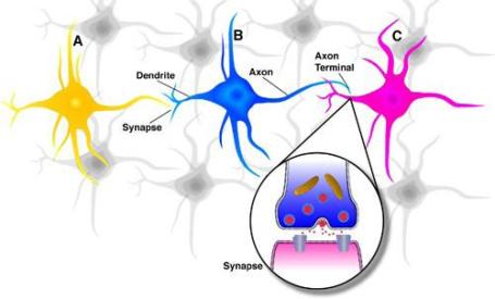
Inputs come into each neuron and then if a weighted sum of the signals it receives is high enough then its outputs will fire (with a certain strength) which will then feed into another layer of neurons. This rather simplistic model of neurons and the brain is what we will model for our initial neural networks.
We will take some sort of vector of inputs and feed them into an input layer of neurons which based on the weighted sums of these inputs will fire with some strength into the next layer of neurons. In neural networks any layers of neurons that aren’t externally connected to inputs or outputs are called hidden layers. The following diagram shows this model.
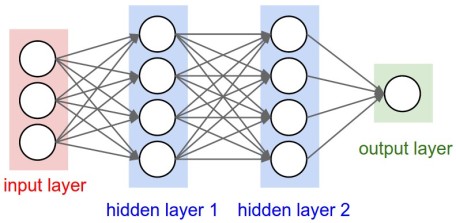
Notice that all the inputs connect to all the next layer of neurons. In a biological brain, there won’t be that many connections, but here when we train this model to determine the weights, some weights will be zero (or very small) corresponding to there not really being a connection. But having a fixed complete set of connections really is just convenience to make the math easier and more uniform.
If you work out the math of doing all these weighted sums you quickly realize, you are just doing matrix algebra and you can get the input to the next layer by multiplying the inputs to this layer by a matrix. So:
Output of Layer = A x (Input of Layer)
Where A is the matrix of weights. That’s simple and easy to calculate (just ignoring for now where the elements of the matrix A come from).
If you remember your matrix algebra you will realize that if you do this to each layer, since this is just linear, you can multiply all the matrixes together and reduce the multiple layer problem to a single layer problem. So in this simple view there is no value in multiple layers. Additionally, linear models are overly simple and can be constructed and solved quite easily. Also with this the output is unbounded, it can come out at any magnitude, which clearly real neurons can’t.
What most neural networks do is add a non-linear activation function to this equation. The activation function maps the output value back into a valid range, adds a non-linearity so the whole equation doesn’t just transform back to one layer as well as adds flexibility in how the model can produce values. The new form of the equation then becomes:
Output of Layer = ActivationFunction( A x (Input of Layer) + b )
Where b is a scalar vector that allows the output to be shifted into range of the activation function. The simplest activation function is the rectifier function defined as f(x) = max( 0, x ). This basically returns x if x is positive and 0 if x is negative. This is good if we only want positive values as output, it is really simple and it does behave like some biological networks. On the downside, it isn’t invertible so we can’t run the network backwards (useful for sanity checking), it isn’t differentiable everywhere (helps with solving for the weights) and it doesn’t provide an upper bound on the output. All that being said, ReLU (Rectified Linear Unit) neural networks are currently the most popular. A smooth version of ReLU is the softplus function f(x) = ln(1+ex). Other choices of activation function include logistic sigmoid (from probability theory) and hyperbolic tangent (tanh) which we will use.
We’re still a bit theoretical at this point, but once we consider what the inputs look like and what we want for an output then we can start to solve for the bits in the middle. If we have good values for the various A matrixes and b vectors then we can see that with some matrix multiplication, addition and simple function evaluation we can get solutions and as it turns out both modern CPUs and especially GPUs are really good at this.
Stock Market Example
We’ll now start looking at this with a simple stock market example to get an idea how this all works. Suppose we want to feed in the last 30 adjusted closing prices for the 30 stocks that compose the Dow Jones index and we want our neural network to output the next day closing prices for these 30 stocks. We will be starting simple to give the basic ideas then we’ll look at making this model more sophisticated. Let’s see how we can go about this.
Our Input Vector
For any Neural Network we have to feed a vector of floating point numbers. So let’s consider feeding in a vector consisting of the last 30 adjusted closing prices of the first Dow component followed by the last 30 adjusted closes of the next component and so on. This means out input vector will contain 900 elements containing the last 30 adjusted closes of each of the 30 Dow stocks.
You can do this but it causes problems because the activation function we are going to use returns values between -1 and 1. Typically neural networks work best with values in this range (or maybe 0 to 1 if only positive values are required). So to make this work you need to normalize the input data to something that works better. We are going to do three things:
- Divide each stocks price by the first price we have in its history so it starts at 1.
- Rather than use the actual stock price, we’ll use the stock price change (of the price normalized by #1).
- If NaN is returned in the historical data, we will back fill it from the next good value. Fortuneately Pandas provides a function to do this:
trainData.fillna(method=’backfill’, inplace=True)
This then puts all the values nicely in range and makes them fairly uniform. The reason for step 3 is that when we go to train the neural network we want to train it with lots of historical data and if we don’t do this we can’t go back very far. Visa, in its current corporate incarnation, only went public in 2008 and then was added to the Dow in 2013 (replacing Bank of America). So there is no Visa historical data from before 2008. Actually I chose tanh as the activation function after switching to price changes, originally I used ReLU with real prices but it tended to be rather unstable.
Our Output Vector
Out output vector will be the next price changes for the 30 Dow component stocks. Then we just need to undo the first normalization above in order to use them.
Summary
This article was a quick introduction to the equations we are going to solve with TensorFlow and what motivates them. We started to look at how we input data into the model and we will continue next time with finding all the various matrix components by framing it as an optimization problem.
The Road to TensorFlow – Part 4: The Stock Market
Introduction
This is the fourth article in my series on Google TensorFlow and we still won’t get to TensorFlow in this article. We’ve covered Linux, Python and various Python libraries so far. Last time we started to use Python libraries to load stock market data ready to feed into some sort of Neural Network model constructed using TensorFlow. In this article we’re going to take a bit of a side trip into looking at a number of issues, theory and logistics around playing with the stock market.
One thing to remember is that this discussion isn’t pure Mathematics. These are all theories that provide some guidance, they might be based on a lot of historical study, but that doesn’t mean they will be true tomorrow, or even that everyone believes them today. One good reference for this stuff is the Udacity course “Machine Learning for Trading”.
Is This a Suitable Problem for AI?
The first question to ask is whether trading stocks is a suitable problem? After all people can’t predict what the stock market will do tomorrow, so why would we think a computer can? Most AI problems, like image recognition or machine translation, know the problem is solvable since people solve these problems. So they know that if they can successfully model what people are doing, then they should be able to get similar results. In this case we are attempting a problem people can’t solve (but some are better at guessing than others), and hoping that fancy algorithms and big data will perhaps give us an edge. This idea could well be a fantasy since predicting the future in general is impossible. It would be nice if we could do as well as a stock picking cat, but that cat did beat a team of professionals.
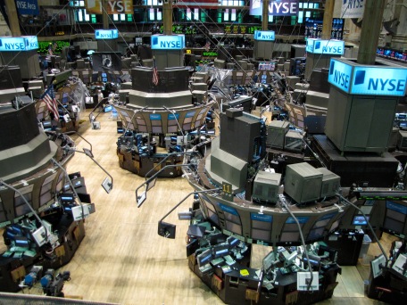
Hedge Funds
Hedge funds are typically high risk funds that perform risky trading strategies for small select clienteles. There are many types of these funds that trade in all sorts of things using all sorts of strategies. However, the ones we are interested in, in this article, are the ones that perform high volume computer trading of stocks. Typically, these are driven by algorithms with little or no human oversight and typically the Hedge fund has an extremely favorable arrangement with a given stock market to allow their computers in the stock markets data center and further that they have extremely low transaction fees. Being in the stock market’s data center means they see everything first since they have no latency. Then don’t have to wait 10ms or whatever for information to make it to your location over the internet. Using very high powered computers they can profit by trading during these latencies (possibly taking your profit).
If these advantages weren’t enough, some Hedge funds have negotiated the right to filter all stock market transactions before they happen and optionally execute the trade themselves again allowing them room to make small profits by inserting themselves into other people’s transactions.
The main takeaway from this, is that unless you are such a Hedge fund, you are at a considerable disadvantage. This is one of the main reasons that day traders have all but disappeared. Hedge funds were able to manipulate them and generally profit from the day traders.
The other thing to remember is that Hedge funds are large and capable of manipulating the market. Often they will play against known trading strategies by over selling or buying to make it look like something is happening and then tricking people into doing things that are a bad idea and profiting from it.
The Efficient Market Hypothesis
The Efficient Market Hypothesis (EMH) states that asset prices fully reflect all available information. There are weaker and stronger forms of this hypothesis, but the basic premise is that you can’t beat the market and you may as well put all your money in an index fund that just matches market performance. Basically that it is futile to try and find undervalued stocks to buy or overvalued stocks to sell.
One claim is that Hedge funds contribute to making the markets efficient. Since they trade so quickly any new information is incorporated into the prices of stocks instantly as far as you can tell. Maybe so, but it does rub the wrong way that someone is profiting this way.
Not everyone believes the EMH, but at the same time it has been proven out time and time again especially in the large heavily traded world markets.
CAPM
This is the Capital Asset Pricing Model that is often used in portfolio management to manage risk, but its also often used in stock trading. A simple form of this equation is:
ri(t) = βi * rm(t) + αi
This says that the return for a given stock i at a point of time t given by ri(t) is equal to a constant βi times the market return at time t given by rm(t) plus a constant αi. Where the expected value of αi is zero. There is usually another term for the base interest rate, but that is effectively zero these days.
The upshot of this is that stocks move with the market and not individually. Each stocks beta can be determined from the stocks history and then this gives a pretty good model for stock returns. This is bad if you have some special insight into a stock, for instance if you are an expert in its industry or perhaps have a good idea of the future trend. For instance if you know something bad is going to happen, you want to short the stock, but if the market goes up that day, it could overwhelm the individual stocks bad news and you lose on your position.
If you believe the EMH then alpha will always be zero or go to zero before you can capitalize on it.
The first Hedge founds came up with a clever scheme to avoid this. If you have two stocks, one you think is going to go up (positive alpha) and another that you think will go down (negative alpha) then you can buy/sell these stocks in pairs by choosing weights of the positions that cause the two beta component to cancel out. This way you eliminate the market from the equation and can concentrate on just the stocks. This is in fact where Hedge funds got their name, using two stocks to hedge their market exposure. This worked for awhile and then others figured out ways to exploit this and it caused a market crash and bailout for a number of funds when it failed. Now this buy/sell pair strategy doesn’t work. As most strategies seem to stop working once they are widely enough known.
Finding alpha is an interesting pursuit. For Hedge funds it could be via illegal insider information as dramatized in the TV series “Billions”. Or it could be via semi-legal methods like hiring a guy in China to sit by the road and could the number of trucks that come out of a factory. Certainly studying Apple’s suppliers and factories is a huge industry in trying to gather information on secretive Apple.
The Fundamental Law of Active Management
The fundamental law of active management is the following:
Performance = skill * square root(breadth)
This basically says that the performance of a portfolio manager is equal to his skill times the square root of the number of trades he makes. This law basically says that a poor portfolio manager can make up for his stupidity via volume.
For instance, Warren Buffet is really smart (high skill) and gets a really great return. His breadth is really small, he just buys 120 stocks and holds them. So his breadth is 120. Suppose a Hedge fund has developed a computer algorithm for stock trading that is 1/1000 as smart as Warren Buffet. Then if you do the math with this formula it comes out that the Hedge fund needs to trade 120,000,000 times a year to match Warren Buffet’s performance. The scary part is that there are lots of Hedge funds that employ this strategy. They have low grade (not very smart) algorithms that can get the same return as Warren Buffet by doing huge numbers of trades.
Adjusted Close
In the previous blog posting we read in the history of adjusted closes for all thirty components of the Dow Jones index. There was also a close price returned, why did we use the adjusted close rather than the real close? If a stock does well, its price goes up and the stock gets too expensive. To help with this every now and then a company will split its stock. They will issue say 2 new stocks for each old stocks. Everyone gets these, then now have twice the stocks at half the price. So from people’s point of view they still have the same value and nothing has changed. Stocks also issue dividends. Whenever a stock does this its prices goes up the value of the dividend before payment and then goes back down right after payment. Again to stock owners this is all well and good and understood. But these two things cause havoc to developing stock market pricing models and algorithms. Without knowing anything else a stock split looks catastrophic. So to help with this, stock markets provide the adjusted close which will adjust historical data for stock splits and dividends so they don’t mess up charts and algorithms. Generally, quite a nice feature of stock feeds. If you compare adjusted close and close they will be the same back to the last event of this nature and at that point will diverge.
Stock Prices
Stock prices don’t by themselves tell you anything about a company and can’t be used to directly compare companies. A company’s value is the stock price times the number of shares. But all companies have issued different numbers of shares and have completely different histories of stock splits, additional share offerings, etc. One way to deal with this is to normalize the stock market data, for instance you could divide all the share prices in a history by the first price. This will cause the stock price to start at 1 and then evolve from there. This does provide one way to compare performance graphically. When doing AI we tend to have to normalize data since the algorithms we are going to use generally don’t like working on large ranges of numbers. We’ll talk more about that later.
Testing with Real Money
We’re not going to test anything with real money. However, most algorithms need real testing in the real market. What we are going to look at doesn’t worry about transaction fees. It also doesn’t worry about some market logistics, since we are only looking at closing prices. You can’t get the previous close price at the next day’s open due to after hours trading and in general how stock order books work. Also if you are a big Hedge fund then actually performing your trades may affect the market. I might have a brilliant algorithm that makes me lots of money in a simulator, but if I run it in the real market, the market may react and counter what I’m doing. Worst sometimes Hedge funds have caused market crashes, or caused the stock market circuit breakers to kick in as a result of their actions.
Summary
This was a really quick introduction to the stock market concepts we’ll be talking about. If you are interested, you can follow the links in the article to learn more.
The Road to TensorFlow – Part 3: Python Libraries
Introduction
Continuing on with my long and winding journey to learn TensorFlow, we started with Linux then went on toPython. Today we will be looking at a number of necessary Python libraries.
My background is Mathematics and I’ve always had an interest in Numerical Analysis and Scientific Computing. But I mostly left these behind when I left University. As I learned Python and started to play with it, among the attendant libraries, I was very pleasantly surprised to find that all my favorite numerical algorithms (and many more). These were now all part of the Python fairly standard libraries. Many of these core libraries are still written in their original Fortran or C code, but are tailored to fit very well into the Python ecosystem. All of this is all open source software and to a certain degree made possible by the good work of the GNU Fortran and C compilers.
These libraries led to quite a few diversions from my primary task of learning TensorFlow, but I found this to be quite a wonderful world to become conversant in.
As I completed the TensorFlow tutorials and an Udacity course, I wanted a different problem to play with rather than the standard image recognition and speech analysis projects that seem pretty standard. To use these, you need quite a bit of data to train your algorithms with, so I thought why not do something with stock market data? After all you can easily get gobs of stock market data via web service calls fairly easily (and freely).
Some Useful Libraries
Here are a few of the libraries that I found useful to help with machine learning and TensorFlow.
Numpy – this is the fundamental Python numerical package that most other libraries are built over. It includes a powerful N dimensional array object, useful linear algebra, Fourier transform, random number capabilities and much more.
Scipy – is built on numpy and includes most numerical algorithms you’ve ever heard of including numerical integration, ODE solvers, optimization, interpolation, special functions and signal processing.
Matplotlib – is a very powerful 2D plotting library that is very useful to use to visualize your results.n
Pandas – was originally written as a library to manipulate stock market data and perform the standard things market technical analysts like to do, but now it markets itself as a general purpose data analysis library.
Sympy – is a library for performing symbolic mathematics. Although I’m not using this in relation to TensorFlow (currently), it is a fascinating tool for performing symbolic algebra and calculus.
IPython – is interactive Python when you program in interactive web based notebooks. A useful tool to play with, but I tend to do my real programming in an IDE. Still if you want to quickly play with something, this is lots of fun.
Pickle – although this is a standard library, I thought I’d highlight it since we are about to use it. This library lets you easily save and load Pythons objects to disk files.
Scikit-learn – is a collection of machine learning algorithms for things like clustering, classification and regression. I.e. neural networks aren’t the only way to accomplish these tasks.
There are many more Python libraries for things like writing GUI programs, performing web requests, processing web data, accessing databases, etc. We’ll talk about those as we need them. Since Python has such a large community of users and contributors there are tons of good web pages, blogs, books courses and forums on all of these. Google is your friend.
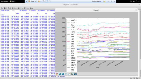
Some Code Finally
So let’s use all of this to load some stock market data which will then be ready for our TensorFlow model. We are going to use Pandas to load some recent prices for the Dow 30 stocks and we’ll use matplotlib to display a graph of their values. This graph is a bit too busy since 30 stocks is also really too many to display at once. Also we haven’t normalized the data at all, so this doesn’t give any real way to compare them. It really only shows we’ve loaded a bunch of data which is hopefully correct.
In this snippet we only load a small bit of history, so its reasonably quick but when we want large amounts of data we will want to cache this. So when we do the web services call to get the data, we pickle it to a file (Python speak for serializing our data object and saving it to a file). If the file exists we just read it from the file and skip the web service call. To refresh the data from the web service, just delete the stocks.pickle file.
We get the data from Yahoo Finance. We could use Yahoo’s Python library directly, but I thought I might use the Pandas DataReader general purpose API to make it easy to switch to Google if Verizon shuts down (or strangles) this service now that they own Yahoo. The Web Services call returns the open, high, low, volume, close and adjusted close which is why we have the couple of lines to clean up the data and only keep the adjusted close. I’ll talk more about the stock market and what the adjusted close is next time.
The program wants to get TrainDataSetSize prices for each stock which is set to 50 below. But due to weekends and holidays, you can’t just subtract 50 from today’s date to get that. So I use a simple heuristic to ensure I get more data than that (which massively overestimates).
import time
import math
import os
from datetime import date
from datetime import timedelta
import numpy as np
import matplotlib
import pandas as pd
import pandas_datareader as pdr
from pandas_datareader import data, wb
from six.moves import cPickle as pickle

TrainDataSetSize = 50

# Load the Dow 30 stocks from Yahoo into a Pandas datasheet

dow30 = ['AXP', 'AAPL', 'BA', 'CAT', 'CSCO', 'CVX', 'DD', 'XOM',
          'GE', 'GS', 'HD', 'IBM', 'INTC', 'JNJ', 'KO', 'JPM',
          'MCD', 'MMM', 'MRK', 'MSFT', 'NKE', 'PFE', 'PG',
          'TRV', 'UNH', 'UTX', 'VZ', 'V', 'WMT', 'DIS']

stock_filename = 'stocks.pickle'
if os.path.exists(stock_filename):
     try:
         with open(stock_filename, 'rb') as f:
             trainData = pickle.load(f)
     except Exception as e:
       print('Unable to process data from', stock_filename, ':', e)
       raise
     print('%s already present - Skipping requesting/pickling.' %
         stock_filename)
else:
     f = pdr.data.DataReader(dow30, 'yahoo', date.today()-
         timedelta(days=TrainDataSetSize*2+5), date.today())
     cleanData = f.ix['Adj Close']
     trainData = pd.DataFrame(cleanData)
     print('Pickling %s.' % stock_filename)
     try:
         with open(stock_filename, 'wb') as f:
           pickle.dump(trainData, f, pickle.HIGHEST_PROTOCOL)
     except Exception as e:
         print('Unable to save data to', stock_filename, ':', e)

print(trainData)

trainData.plot()
matplotlib.pyplot.show()
Generally, I think this is a fairly short bit of code that accomplishes all this. This is one of the beauties of Python that it is so compact.
Summary
This was a quick introduction the Python libraries we’ll be using in addition to TensorFlow. Hopefully the quick sample program gave a taste of how we will be using them and is in fact how we will be getting training data for our TensorFlow model.
The Road to TensorFlow – Part 2: Python
Introduction
This is part 2 on my blog series on playing with TensorFlow. Last time I blogged on getting Linux going in a VM. This time we will be talking about the Python programming language. The API for TensorFlow is primarily aimed at Python and in fact much of the research in AI, scientific computing, numerical computing and data research all takes place in Python. There is a C++ API as well, but it seems like a good chance to give Python a try.
Python is an interpreted language that is very rich in supporting various programming paradigms like object oriented, procedural and functional. Python is open source and runs on many platforms. Most Linux’s and the MacOS come with some version of Python pre-installed. Python is very interoperable and can work with most other programming systems, and there are a huge number of libraries of functionality available to the Python programmer. Python is oriented to getting things done quickly with a minimum of code and a minimum of fuss. The name Python is a tribute to the comedy troupe Monty Python and there are many references to Monty Python throughout the documentation.

Installation and Versions
Although I generally like Python it has one really big problem that is generally a pain in the ass when setting up new systems and browsing documentation. The newest version of Python as of this writing is 3.5.2 which is the one I wanted to use along with all the attendant libraries. However, if you type python in a terminal window you get 2.7.12. This is because when Python went to version 3 it broke source code compatibility. So they made the decision to maintain version 2 going forwards while everyone updated their programs and scripts to version 3. Version 3.0 was released in 2008 and this mess is still going on eight years later. The latest Python 2.x, namely 2.7.12 was just released in June 2016 and seems to be quite actively developed by a good sized community. So generally to get anything Python 3.x you need to add a 3 to the end. So to run Python 3.5.2 in a terminal window you type python3. Similarly, the IDE is IDLE3 and the package installer is pip3. It makes it very easy to make a mistake an to get the wrong thing. Worse the naming isn’t entirely consistent across all packages, there are several that I’ve run into where you add a 2 for the 2.x version and the version 3 one is just the name. As a result, I always get a certain amount of Python 2.x stuff accidentally installed by mistake (which doesn’t hurt anything, just wastes time and disk space). This also leads to a bit of confusion when you Google for information, in that you have to be careful to get 3.x info rather than 2.x info as the wrong one may or may not work and may or may not be a best practice.
On Ubuntu Linux I just used apt-get to install the various packages I needed. I’ll talk about these a bit more in the next posting. Another option for installing Python and all the scientific libraries is to use the Anacondadistribution which is quite a good way to get everything in Python installed all at once. I used Anaconda to install Python on Windows 10 at it worked really well, you just don’t get the fine control of what it does and it creates a separate installation to keep everything separate from anything already installed.
Python the Language
Python is a very large language; it has everything from object orientation to functional programming to huge built in libraries. It does have a number of quirks though. For instance, the way you define blocks is via indentation rather than using curly brackets or perhaps end block statements. So indentation isn’t just a style guideline, it’s fundamental to how the program works. In the following bit of code:
for i in range(10):
a = i * 8
print( i, a )
a = 8
the two indented statements are part of the for loop and the out-dented assignment is outside the loop. You don’t define variables, they are defined when first assigned to, and you can’t use a variable without assigning it first (or an exception will be thrown). There are a lot of built in types including dictionaries and lists, but no array type (but the numpy library does add these). Notice how the for loop uses in rather than to, to do a basic loop.
I don’t want to get too much into the language since it is quite large. If you are interested there are many good sites on the web to teach Python and the O’Reilly book “Learning Python” is recommended (but quite long).
Since Python is interpreted, you don’t need to wait for any compile steps so the coding, testing, debugging cycle is quite quick. Writing tight loops in Python will be slower than C, but generally Python gives you quite good libraries to do most of what you want and the libraries tend to be written in C or Fortran and very fast. So far I haven’t found speed to be an issue. TensorFlow is also written in C for speed, plus it has the ability to run on NVidia graphics cards for an extra boost.
Summary
This was my quick intro to Python. I’ll talk more about relevant parts of Python as I go along in this series. I generally like Python and so far my only big complaint is the confusion between the version 2 world and the version 3 world.
The Road to TensorFlow – Part 1 Linux
Introduction
There have been some remarkable advancements in Artificial Intelligence type algorithms lately. I blogged on this a little while ago here. Whether its computers reading hand-writing, understanding speech, driving cars or winning at games like Go, there seems to be a continual flood of stories of new amazing accomplishments. I thought I’d spend a bit of time getting to know how this was all coming about by doing a bit of reading and playing with the various technologies.
I wanted to play with Neural Network technology, so thought the Google TensorFlow open source toolkit would be a good place to start. This led me down the road to quite a few new (to me) technologies. So I thought I’d write a few blog posts on my road to getting some working TensorFlow programs. This might take quite a few articles covering Linux, Python, Python libraries like Pandas, Stock Market technical analysis, and then TensorFlow.
Linux
The first obstacle I ran into was that TensorFlow had no install image for Windows, after a bit of Googling, I found you need to run it on MacOS or Linux. I haven’t played with Linux in a few years and I’d been meaning to give it a try.
I happened to have just read about a web site osboxes.org that provides VirtualBox and VMWare images of all sorts of versions of Linux all ready to go. So I thought I’d give this a try. I downloaded and installed VirtualBox and downloaded a copy of 64Bit Ubuntu Linux. Since I didn’t choose anything special I got Canonical’s Unity Desktop. Since I was trying new things, I figured oh well, lets get going.
Things went pretty well at first, I figured out how to install things on Ubuntu which uses APT (Advanced Packaging Tool) which is a command line utility to install things into Ubuntu Linux. This worked pretty well and the only problems I had were particular to installing Python which I’ll talk about when I get to Python. I got TensorFlow installed and was able to complete the tutorial, I got the IDLE3 IDE for Python going and all seemed good and I felt I was making good progress.
Then Ubuntu installed an Ubuntu update for me (which like Windows is run automatically by default). This updated many packages on my virtual image. And in the process broke the Unity desktop. Now the desktop wouldn’t come up and all I could do was run a single terminal window. So at least I could get my work off the machine. I Googled the problem and many people had it, but none of the solutions worked for me and I couldn’t resolve the problem. I don’t know if its just that Unity is finicky and buggy or if it’s a problem with running in a VirtualBox VM. Perhaps something with video drivers, who knows.
Anyway I figured to heck with Ubuntu and switched to Red Hat’s Fedora Linux. I chose a standard simpleGnome desktop and swore to never touch Unity again. I also realized that now I’m retired, I’m not a commercial user, so I can freely use VMWare, so I also switched to VMWare since I wondered if my previous problem was caused by VirtualBox. Anyway installing TensorFlow on Fedora seemed to be quite difficult. The dependencies in the TensorFlow install assume the packages that Ubuntu installs by default and apparently these are quite different that Fedora. So after madly installing things that I didn’t really think were necessary (like the Gnu Fortran compiler), I gave up on Fedora.
So I went back to osboxes.org and downloaded an Ubuntu image with the Gnome desktop. This then has been working great. I got everything re-installed quite quickly and was back to being productive. I like Gnome much better than Unity and I haven’t had any problems. Similarly, I think VMWare works a bit better than VirtalBox and I think I get a bit better performance in this configuration.
I have Python along with all the Python scientific and numerical computing libraries working. I have TensorFlow working. I spend most of my time in Terminal windows and the IDLE3 IDE, but occasionally use FireFox and some of the other programs pre-installed with the distribution.
I’m greatly enjoying working with Linux again, and I’m considering replacing my currently broken desktop computer with something inexpensive natively running Linux. I haven’t really enjoyed the direction Windows has taken after Windows 7 and I’m thinking of perhaps doing most of my computing on Linux and MacOS.
Summary
I am enjoying using Linux again. In spite of my initial problems with Ubuntu’s Unity Desktop and then with Fedora (running TensorFlow). Now that I have a good system that seems to be stable and working well I’m pretty happy with it. I’m also glad to be free of things like App stores and its nice to feel in control of my environment when running Linux. Anyway this was the small first step to TensorFlow.