续集请点击我:tensorflow学习笔记——使用TensorFlow操作MNIST数据(2)
本节开始学习使用tensorflow教程,当然从最简单的MNIST开始。这怎么说呢,就好比编程入门有Hello World,机器学习入门有MNIST。在此节,我将训练一个机器学习模型用于预测图片里面的数字。
开始先普及一下基础知识,我们所说的图片是通过像素来定义的,即每个像素点的颜色不同,其对应的颜色值不同,例如黑白图片的颜色值为0到255,手写体字符,白色的地方为0,黑色为1,如下图。
MNIST 是一个非常有名的手写体数字识别数据集,在很多资料中,这个数据集都会被用做深度学习的入门样例。而Tensorflow的封装让MNIST数据集变得更加方便。MNIST是NIST数据集的一个子集,它包含了60000张图片作为训练数据,10000张图片作为测试数据。在MNIST数据集中的每一张图片都代表了0~9中的一个数字。图片的大小都为28*28,且数字都会出现在图片的正中间,如下图:

在上图中右侧显示了一张数字1的图片,而右侧显示了这个图片所对应的像素矩阵,MNIST数据集提供了四个下载文件,在tensorflow中可以将这四个文件直接下载放到一个目录中并加载,如下代码input_data.read_data_sets所示,如果指定目录中没有数据,那么tensorflow会自动去网络上进行下载。下面代码介绍了如何使用tensorflow操作MNIST数据集。
MNIST数据集的官网是Yann LeCun's website。在这里,我们提供了一份python源代码用于自动下载和安装这个数据集。你可以下载这份代码,然后用下面的代码导入到你的项目里面,也可以直接复制粘贴到你的代码文件里面。
注意:MNIST数据集包括训练集的图片和标记数据,以及测试集的图片和标记数据,在测试集包含的10000个样例中,前5000个样例取自原始的NIST训练集,后5000个取自原始的NIST测试集,因此前5000个预测起来更容易些。
import tensorflow.examples.tutorials.mnist.input_data as input_data
mnist = input_data.read_data_sets("MNIST_data/", one_hot=True)
当one-hot变为为TRUE,则只要对应的位置的值为1,其余都是0。
这里,我直接下载了数据集,并放在了我的代码里面。测试如下:
# _*_coding:utf-8_*_

from tensorflow.examples.tutorials.mnist import input_data

mnist = input_data.read_data_sets('MNIST_data', one_hot=True)
print("OK")
# 打印“Training data size: 55000”
print("Training data size: ", mnist.train.num_examples)
# 打印“Validating data size: 5000”
print("Validating data size: ", mnist.validation.num_examples)
# 打印“Testing data size: 10000”
print("Testing data size: ", mnist.test.num_examples)
# 打印“Example training data: [0. 0. 0. ... 0.380 0.376 ... 0.]”
print("Example training data: ", mnist.train.images[0])
# 打印“Example training data label: [0. 0. 0. 0. 0. 0. 0. 1. 0. 0.]”
print("Example training data label: ", mnist.train.labels[0])

batch_size = 100
# 从train的集合中选取batch_size个训练数据
xs, ys = mnist.train.next_batch(batch_size)
# 输出“X shape:(100,784)”
print("X shape: ", xs.shape)
# 输出"Y shape:(100,10)"
print("Y shape: ", ys.shape)
结果如下:
Extracting MNIST_data	rain-images-idx3-ubyte.gz
Extracting MNIST_data	rain-labels-idx1-ubyte.gz
Extracting MNIST_data	10k-images-idx3-ubyte.gz
Extracting MNIST_data	10k-labels-idx1-ubyte.gz
OK
Training data size:  55000
Validating data size:  5000
Testing data size:  10000
X shape:  (100, 784)
Y shape:  (100, 10)
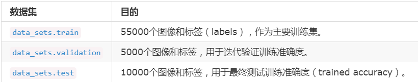
从上面的代码可以看出,通过input_data.read_data_sets函数生成的类会自动将MNIST数据集划分成train,validation和test三个数据集,其中train这个集合内含有55000张图片,validation集合内含有5000张图片,这两个集合组成了MNIST本身提供的训练数据集。test集合内有10000张图片,这些图片都来自与MNIST提供的测试数据集。处理后的每一张图片是一个长度为784的一维数组,这个数组中的元素对应了图片像素矩阵中的每一个数字(28*28=784)。因为神经网络的输入是一个特征向量,所以在此把一张二维图像的像素矩阵放到一个一维数组中可以方便tensorflow将图片的像素矩阵提供给神经网络的输入层。像素矩阵中元素的取值范围为[0, 1],它代表了颜色的深浅。其中0表示白色背景,1表示黑色前景。
Softmax回归的再复习
我们知道MNIST的每一张图片都表示一个数字,从0到9。我们希望得到给定图片代表每个数字的概率。比如说,我们的模型可能推测一张包含9的图片代表数字9 的概率为80%但是判断它是8 的概率是5%(因为8和9都有上半部分的小圆),然后给予它代表其他数字的概率更小的值。
这是一个使用softmax regression模型的经典案例。softmax模型可以用来给不同的对象分配概率。即使在之后,我们训练更加精细的模型的时候,最后一步也是需要softmax来分配概率。
Softmax回归可以解决两种以上的分类,该模型是Logistic回归模型在分类问题上的推广。对于要识别的0~9这10类数字,首选Softmax回归。MNIST的Softmax回归源代码位于Tensorflow-1.1.0/tensorflow.examples/tutorials/mnist/mnist_softmax.py
softmax回归第一步
为了得到一张给定图片属于某个特定数字类的证据(evidence),我们对图片像素值进行加权求和。如果这个像素具有很强的证据说明这种图片不属于该类,那么相应的权值为负数,相反如果这个像素拥有很强的证据说明这张图片不属于该类,那么相应的权值为负数,相反如果这个像素拥有有力的证据支持这张图片属于这个类,那么权值是正数。
下面的图片显示了一个模型学习到的图片上每个像素对于特定数字类的权值,红色代表负数权值,蓝色代表正数权值。
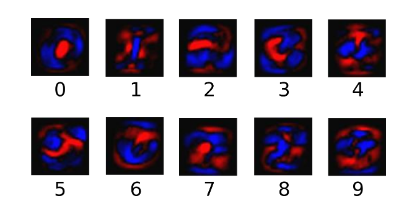
我们也需要加入一个额外的偏置量(bias),因为输入往往会带有一些无关的干扰量。因为对于给定的输入图片 x 它代表的是数字 i 的证据可以表示为:
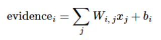
其中,Wi代表权重,bi代表数字 i 类的偏置量, j 代表给定图片 x 的像素索引用于像素求和。然后用 softmax 函数可以把这些证据转换成概率 y:
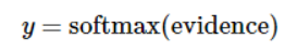
这里的softmax可以看成是一个激励(activation)函数或者链接(link)函数,把我们定义的线性函数的输出转换成我们想要的格式,也就是关于10个数字类的概率分布。因此,给定一张图片,它对于每一个数字的吻合度可以被softmax函数转换成一个概率值。softmax函数可以定义为:
![]()
展开等式右边的子式,可以得到:

但是更多的时候把softmax模型函数定义为前一种形式:把输入值当做幂指函数求值,再正则化这些结果值。这个幂运算表示,更大的证据对应更大的假设模型(hypothesis)里面的乘数权重值。反之,拥有更少的证据意味着在假设模型里面拥有更小的乘数系数。假设模型里面的权值不可以是0值或者负值。Softmax然后会正则化这些权重值,使他们的总和等于1,以此构造一个有效的概率分布。
对于softmax回归模型可以用下面的图解释,对于输入的 xs 加权求和,再分别加上一个偏置量,最后再输入到 softmax 函数中:
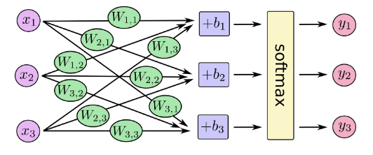
如果把它写成一个等式,我们可以得到:
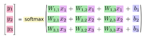
我们也可以用向量表示这个计算过程:用矩阵乘法和向量相加。这有助于提高计算效率:

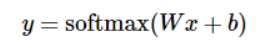
更进一步,可以写成更加紧凑的方式:
接下来就是使用Tensorflow实现一个 Softmax Regression。其实在Python中,当还没有TensorFlow时,通常使用Numpy做密集的运算操作。因为Numpy是使用C和一部分 fortran语言编写的,并且调用了 openblas,mkl 等矩阵运算库,因此效率很好。其中每一个运算操作的结果都要返回到Python中,但不同语言之间传输数据可能会带来更大的延迟。TensorFlow同样将密集的复杂运算搬到Python外面执行,不过做的更彻底。
首先载入TensorFlow库,并创建一个新的 InteractiveSession ,使用这个命令会将这个session 注册为默认的session,之后的运算也默认跑在这个session里,不同session之间的数据和运算应该都是相互独立的。接下来创建一个 placeholder,即输入数据的地方。Placeholder 的第一个参数是数据类型,第二个参数 [None, 784] 代表 tensor 的 shape,也就是数据的尺寸,这里的None代表不限条数的输入, 784代表每条数据的是一个784维的向量。
sess = tf.InteractiveSession()
x = tf.placeholder(tf.float32, [None, 784])
接下来要给Softmax Regression模型中的 weights和 biases 创建 Variable 对象,Variable是用来存储模型参数的,不同于存储数据的 tensor 一旦使用掉就会消失,Variable 在模型训练迭代中是持久的,它可以长期存在并且在每轮迭代中被更新。我们把 weights 和 biases 全部初始化为0,因为模型训练时会自动学习适合的值,所以对这个简单模型来说初始值不太重要,不过对于复杂的卷积网络,循环网络或者比较深的全连接网络,初始化的方法就比较重要,甚至可以说至关重要。注意这里的W的shape是 [784, 10] 中 , 784是特征的维数,而后面的10 代表有10类,因为Label在 one-hot编码后是10维的向量。
W = tf.Variable(tf.zeros([784, 10]))
b = tf.Variable(tf.zeros([10]))
接下来要实现 Softmax Regression 算法,我们将上面提到的 y = softmax(Wx+b),改为 TensorFlow的语言就是下面的代码:
y = tf.nn.softmax(tf.matmul(x, W) + b)
Softmax是 tf.nn 下面的一个函数,而 tf.nn 则包含了大量的神经网络的组件, tf.matmul是TensorFlow中矩阵乘法函数。我们就定义了简单的 Softmax Regression,语法和直接写数学公式很像。然而Tensorflow最厉害的地方还不是定义公式,而是将forward和backward的内容都自动实现。所以我们接下来定义好loss,训练时将会自动求导并进行梯度下降,完成对 Softmax Regression模型参数的自动学习。
回归模型训练的步骤
构建回归模型,我们需要输入原始真实值(group truth),计算采用softmax函数拟合后的预测值,并定义损失函数和优化器。
为了训练模型,我们首先需要定义一个指标来评估这个模型是好的。其实,在机器学习中,我们通常定义指标来表示一个模型是坏的,这个指标称为成本(cost)或者损失(loss),然后近邻最小化这个指标。但是这两种方式是相同的。
一个非常常见的的成本函数是“交叉熵(cross-entropy)”。交叉熵产生于信息论里面的信息压缩编码技术,但是后来他演变为从博弈论到机器学习等其他领域里的重要技术手段,它的定义如下:

Y是我们预测的概率分布, y' 是实际的分布(我们输入的 one-hot vector)。比较粗糙的理解是,交叉熵是用来衡量我们的预测用于描述真相的低效性。
为了计算交叉熵,我们首先需要添加一个新的占位符用于输入正确值:
y_ = tf.placeholder("float", [None,10])
然后我们可以用交叉熵的公式计算交叉熵:
cross_entropy = -tf.reduce_sum(y_*tf.log(y))
或者
cross_entropy = tf.reduce_mean(-tf.reduce_sum(y_ * tf.log(y),
                                              reduction_indices=[1]))
(这里我们 y_ * tf.log(y)是前面公式的交叉熵公式,而 tf.reduce_sum就是求和,而tf.reduce_mean则是用来对每个 batch 的数据结果求均值。)
首先,用 tf.log 计算 y 的每个元素的对数。接下来,我们把 y_ 的每一个元素 和 tf.log(y) 的对应元素相乘。最后用 tf.reduce_sum 计算张量的所有元素总和。(注意:这里的交叉熵不仅仅用来衡量单一的一对预测和真实值,而是所有的图片的交叉熵的总和。对于所有的数据点的预测表现比单一数据点的表现能更好的描述我们的模型的性能)。
当我们知道我们需要我们的模型做什么的时候,用TensorFlow来训练它是非常容易的。因为TensorFlow拥有一张描述我们各个计算单元的图,它可以自动的使用反向传播算法(backpropagation algorithm)来有效的确定变量是如何影响想要最小化的那个成本值。然后TensorFlow会用选择的优化算法来不断地修改变量以降低成本。
train_step = tf.train.GradientDescentOptimizer(0.01).minimize(cross_entropy)
在这里,我们要求TensorFlow用梯度下降算法(gradient descent alogrithm)以0.01的学习速率最小化交叉熵。梯度下降算法(gradient descent algorithm)是一个简单的学习过程,TensorFlow只需将每个变量一点点地往使成本不断降低的方向移动。当然TensorFlow也提供了其他许多优化算法:只要简单地调整一行代码就可以使用其他的算法。
TensorFlow在这里实际上所做的是,它会在后台给描述你的计算的那张图里面增加一系列新的计算操作单元用于实现反向传播算法和梯度下降算法。然后,它返回给你的只是一个单一的操作,当运行这个操作时,它用梯度下降算法训练你的模型,微调你的变量,不断减少成本。
现在,我们已经设置好了我们的模型,在运行计算之前,我们需要添加一个操作来初始化我们创建的变量并初始化,但是我们可以在一个Session里面启动我们的模型:
with tf.Session() as sess:
    tf.global_variables_initializer().run()
然后开始训练模型,这里我们让模型训练训练1000次:
for i in range(1000):
  batch_xs, batch_ys = mnist.train.next_batch(100)
  sess.run(train_step, feed_dict={x: batch_xs, y_: batch_ys})
或者
for i in range(1000):
    batch_xs, batch_ys = mnist.train.next_batch(100)
    train_step.run({x: batch_xs, y:batch_ys})
该训练的每个步骤中,我们都会随机抓取训练数据中的100个批处理数据点,然后我们用这些数据点作为参数替换之前的占位符来运行 train_step。而且我们可以通过 feed_dict 将 x 和 y_ 张量 占位符用训练数据替代。(注意:在计算图中,我们可以用 feed_dict 来替代任何张量,并不仅限于替换占位符)
使用一小部分的随机数据来进行训练被称为随机训练(stochastic training)- 在这里更确切的说是随机梯度下降训练。在理想情况下,我们希望用我们所有的数据来进行每一步的训练,因为这能给我们更好的训练结果,但显然这需要很大的计算开销。所以,每一次训练我们可以使用不同的数据子集,这样做既可以减少计算开销,又可以最大化地学习到数据集的总体特性。
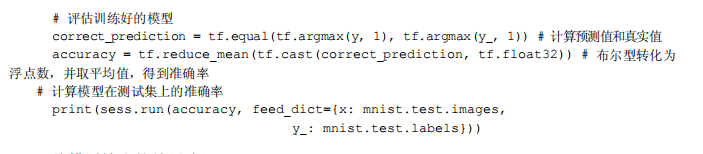
现在我们已经完成了训练,接下来就是对模型的准确率进行验证,下面代码中的 tf.argmax是从一个 tensor中寻找最大值的序号, tf.argmax(y, 1)就是求各个预测的数字中概率最大的一个,而 tf.argmax(y_, 1)则是找到样本的真实数字类别。而 tf.equal方法则是用来判断预测数字类别是否就是正确的类别,最后返回计算分类是否正确的操作 correct_predition。
训练模型的步骤
已经设置好了模型,在训练之前,需要先初始化我们创建的变量,以及在会话中启动模型。
# 这里使用InteractiveSession() 来创建交互式上下文的TensorFlow会话
# 与常规会话不同的时,交互式会话成为默认会话方法
# 如tf.Tensor.eval 和 tf.Operation.run 都可以使用该会话来运行操作(OP
sess = tf.InteractiveSession()
tf.global_variables_initializer().run()
我们让模型循环训练1000次,在每次循环中我们都随机抓取训练数据中100个数据点,来替代之前的占位符。
# Train
for _ in range(1000):
    batch_xs, batch_ys = mnist.train.next_batch(100)
    sess.run(train_step, feed_dict={x:batch_xs, y_:batch_ys})
这种训练方式成为随机训练(stochastic training),使用SGD方法进行梯度下降,也就是每次从训练数据集中抓取一小部分数据进行梯度下降训练。即与每次对所有训练数据进行计算的BGD相比,SGD即能够学习到数据集的总体特征,又能够加速训练过程。
保存检查点(checkpoint)的步骤
为了得到可以用来后续恢复模型以进一步训练或评估的检查点文件(checkpoint file),我们实例化一个 tf.train.Saver。
saver = tf.train.Saver()
在训练循环中,将定期调用 saver.save() 方法,向训练文件夹中写入包含了当前所有可训练变量值的检查点文件。
saver.save(sess, FLAGS.train_dir, global_step=step)
这样,我们以后就可以使用 saver.restore() 方法,重载模型的参数,继续训练。
saver.restore(sess, FLAGS.train_dir)
这里不多讲,具体请参考博客:TensorFlow学习笔记:模型持久化的原理。。
评估模型的步骤
那么我们的模型性能如何呢?
首先让我们找出那些预测正确的标签。tf.argmax 是一个非常有用的函数,它能给出某个 tensor 对象在某一维上的其数据最大值所在的索引值。由于标签向量是由0, 1 组成,所以最大值1所在的索引位置就是类别标签,比如 tf.argmax(y, 1) 返回的是模型对于任一输入 x 预测到的标签值,而 tf.argmax(y_, 1) 代表正确的标签,我们可以用 tf.equal 来检测我们的预测是否真实标签匹配(索引位置一样表示匹配)。
correct_prediction = tf.equal(tf.argmax(y,1), tf.argmax(y_,1))
这里返回一个布尔数组,为了计算我们分类的准确率,我们使用cast将布尔值转换为浮点数来代表对,错,然后取平均值。例如: [True, False, True, True] 变为 [1, 0, 1, 1],计算出平均值为 0.75。
accuracy = tf.reduce_mean(tf.cast(correct_prediction, "float"))
最后,我们可以计算出在测试数据上的准确率,大概是91%。
print(accuracy.eval(feed_dict={x: mnist.test.images, y_: mnist.test.labels}))
完整代码如下:
下面我们总结一下实现了上面简单机器学习算法 Softmax Regression,这可以算作是一个没有隐含层的最浅的神经网络,我们来总结一下整个流程,我们做的事情分为下面四部分:
- 1,定义算法公式,也就是神经网络forward时的计算
- 2,定义loss,选定优化器,并指定优化器优化loss
- 3,迭代地对数据进行训练
- 4,在测试集或验证集上对准确率进行评测
这几个步骤是我们使用Tensorflow进行算法设计,训练的核心步骤,也将会贯穿所有神经网络。
代码如下:
#_*_coding:utf-8_*_
import tensorflow as tf
from tensorflow.examples.tutorials.mnist import input_data

# 首先我们直接加载TensorFlow封装好的MNIST数据   28*28=784
mnist = input_data.read_data_sets('MNIST_data/', one_hot=True)
print(mnist.train.images.shape, mnist.train.labels.shape)
print(mnist.test.images.shape, mnist.test.labels.shape)
print(mnist.validation.images.shape, mnist.validation.labels.shape)
'''
(55000, 784) (55000, 10)
(10000, 784) (10000, 10)
(5000, 784) (5000, 10)
'''

sess = tf.InteractiveSession()
x = tf.placeholder(tf.float32, [None, 784])

W = tf.Variable(tf.zeros([784, 10]))
b = tf.Variable(tf.zeros([10]))

y = tf.nn.softmax(tf.matmul(x, W) + b)

y_ = tf.placeholder(tf.float32, [None, 10])
cross_entropy = tf.reduce_mean(-tf.reduce_sum(y_ * tf.log(y),
                                              reduction_indices=[1]))

train_step = tf.train.GradientDescentOptimizer(0.5).minimize(cross_entropy)

tf.global_variables_initializer().run()

for i in range(1000):
    batch_xs, batch_ys = mnist.train.next_batch(100)
    train_step.run({x: batch_xs, y_: batch_ys})

correct_prediction = tf.equal(tf.argmax(y, 1), tf.argmax(y_, 1))

accuracy = tf.reduce_mean(tf.cast(correct_prediction, tf.float32))

print(accuracy.eval(feed_dict={x: mnist.test.images, y_: mnist.test.labels}))
传统神经网络训练MNIST数据
1,训练步骤
- 输入层:拉伸的手写文字图像,维度为 [-1, 28*28]
- 全连接层:500个节点,维度为[-1, 500]
- 输出层:分类输出,维度为 [-1, 10]
2,训练代码及其结果
传统的神经网络训练代码:
# _*_coding:utf-8_*_
import tensorflow as tf
import numpy as np
from tensorflow.examples.tutorials.mnist import input_data

BATCH_SIZE = 100  # 训练批次
INPUT_NODE = 784  # 784=28*28 输入节点
OUTPUT_NODE = 10  # 输出节点
LAYER1_NODE = 784  # 层级节点
TRAIN_STEP = 10000  # 训练步数
LEARNING_RATE = 0.01
L2NORM_RATE = 0.001


def train(mnist):
    # define input placeholder
    # None表示此张量的第一个维度可以是任何长度的
    input_x = tf.placeholder(tf.float32, [None, INPUT_NODE], name='input_x')
    input_y = tf.placeholder(tf.float32, [None, OUTPUT_NODE], name='input_y')

    # define weights and biases
    w1 = tf.Variable(tf.truncated_normal(shape=[INPUT_NODE, LAYER1_NODE], stddev=0.1))
    b1 = tf.Variable(tf.constant(0.1, shape=[LAYER1_NODE]))

    w2 = tf.Variable(tf.truncated_normal(shape=[LAYER1_NODE, OUTPUT_NODE], stddev=0.1))
    b2 = tf.Variable(tf.constant(0.1, shape=[OUTPUT_NODE]))

    layer1 = tf.nn.relu(tf.nn.xw_plus_b(input_x, w1, b1))
    y_hat = tf.nn.xw_plus_b(layer1, w2, b2)
    print("1 step ok!")

    # define loss
    cross_entropy = tf.nn.softmax_cross_entropy_with_logits(logits=y_hat, labels=input_y)
    cross_entropy_mean = tf.reduce_mean(cross_entropy)
    regularization = tf.nn.l2_loss(w1) + tf.nn.l2_loss(w2) + tf.nn.l2_loss(b1) + tf.nn.l2_loss(b2)
    loss = cross_entropy_mean + L2NORM_RATE * regularization
    print("2 step ok")

    # define accuracy
    correct_predictions = tf.equal(tf.argmax(y_hat, 1), tf.argmax(input_y, 1))
    accuracy = tf.reduce_mean(tf.cast(correct_predictions, tf.float32))
    print("3 step ok")

    # train operation
    global_step = tf.Variable(0, trainable=False)
    train_op = tf.train.AdamOptimizer(LEARNING_RATE).minimize(loss, global_step=global_step)
    print("4 step ok ")

    with tf.Session() as sess:
        tf.global_variables_initializer().run()  # 初始化创建的变量
        print("5 step OK")

        # 开始训练模型
        for i in range(TRAIN_STEP):
            xs, ys = mnist.train.next_batch(BATCH_SIZE)
            feed_dict = {
                input_x: xs,
                input_y: ys,
            }
            _, step, train_loss, train_acc = sess.run([train_op, global_step, loss, accuracy], feed_dict=feed_dict)
            if (i % 100 == 0):
                print("After %d steps, in train data, loss is %g, accuracy is %g." % (step, train_loss, train_acc))

        test_feed = {input_x: mnist.test.images, input_y: mnist.test.labels}
        test_acc = sess.run(accuracy, feed_dict=test_feed)
        print("After %d steps, in test data, accuracy is %g." % (TRAIN_STEP, test_acc))


if __name__ == '__main__':
    mnist = input_data.read_data_sets("data", one_hot=True)
    print("0 step ok!")
    train(mnist)
结果如下:
Extracting data	rain-images-idx3-ubyte.gz
Extracting data	rain-labels-idx1-ubyte.gz
Extracting data	10k-images-idx3-ubyte.gz
Extracting data	10k-labels-idx1-ubyte.gz
0 step ok!
1 step ok!
2 step ok
3 step ok
4 step ok
5 step OK
After 1 steps, in train data, loss is 5.44352, accuracy is 0.03.
After 101 steps, in train data, loss is 0.665012, accuracy is 0.95.

...  ...

After 9901 steps, in train data, loss is 0.304703, accuracy is 0.96.
After 10000 steps, in test data, accuracy is 0.9612.
3,部分代码解析:
占位符
我们通过为输入图像和目标输出类别创建节点,来开始构建计算图:
x = tf.placeholder("float", [None, 784])
x 不是一个特定的值,而是一个占位符 placeholder,我们在TensorFlow运行计算时输入这个值我们希望能够输入任意数量的MNIST图像,每张图展平为784维(28*28)的向量。我们用二维的浮点数张量来表示这些图,这个张量的形状是 [None, 784],这里的None表示此张量的第一个维度可以是任意长度的。
虽然palceholder 的shape参数是可选的,但是有了它,TensorFlow能够自动捕捉因数据维度不一致导致的错误。
变量
一个变量代表着TensorFlow计算图中的一个值,能够在计算过程中使用,甚至进行修改。在机器学习的应用过程中,模型参数一般用Variable来表示。
w1 = tf.Variable(tf.truncated_normal(shape=[INPUT_NODE, LAYER1_NODE], stddev=0.1))
b1 = tf.Variable(tf.constant(0.1, shape=[LAYER1_NODE]))
我们的模型也需要权重值和偏置量,当然我们可以将其当做是另外的输入(使用占位符),这里使用Variable。一个Variable代表一个可修改的张量,它可以用于计算输入值,也可以在计算中被修改。对于各种机器学习英语,一般都会有模型参数,可以用Variable来表示。
变量需要通过session初始化后,才能在session中使用,这一初始化的步骤为,为初始化指定具体值,并将其分配给每个变量,可以一次性为所有变量完成此操作。
sess.run(tf.initialize_all_variables())
卷积神经网络-CNN训练MNIST数据
在MNIST上只有96%的正确率是在是糟糕,所以这里我们用一个稍微复杂的模型:卷积神经网络来改善效果,这里大概会达到100%的准确率。
同样,构建的流程也是先加载数据,再构架网络模型,最后训练和评估模型。
1,训练步骤
- 输入层:手写文字图像,维度为[-1, 28, 28, 1]
- 卷积层1:filter的shape为5*5*32,strides为1,padding为“SAME”。卷积后维度为 [-1, 28, 28, 32]
- 池化层2:max-pooling,ksize为2*2, 步长为2,池化后维度为 [-1, 14, 14, 32]
- 卷积层3:filter的shape为5*5*64,strides为1,padding为“SAME”。卷积后维度为 [-1, 14, 14, 64]
- 池化层4:max-pooling,ksize为2*2, 步长为2。池化后维度为 [-1, 7, 7, 64]
- 池化后结果展开:将池化层4 feature map展开, [-1, 7, 7, 64] ==> [-1, 3136]
- 全连接层5:输入维度 [-1, 3136],输出维度 [-1, 512]
- 全连接层6:输入维度 [-1, 512],输出维度[-1, 10]。经过softmax后,得到分类结果。
2,构建模型
构建一个CNN模型,需要以下几步。
(1)定义输入数据并预处理数据。这里,我们首先读取数据MNIST,并分别得到训练集的图片和标记的矩阵,以及测试集的图片和标记的矩阵。代码如下:
# _*_coding:utf-8_*_
import tensorflow as tf
import numpy as np
from tensorflow.examples.tutorials.mnist import input_data

mnist = input_data.read_data_sets('MNIST_data', one_hot=True)
trX, trY = mnist.train.images, mnist.train.labels
teX, teY = mnist.test.images, mnist.test.labels
其中,mnist是TensorFlow的TensorFlow.contrib.learn中的Datasets,其值如下:

trX, trY, teX, teY 是数据的矩阵表现,其值类似于:
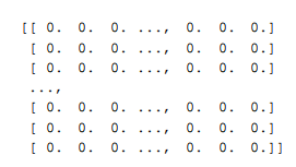
接着,需要处理输入的数据,把上面 trX 和 teX 的形状变为 [-1, 28, 28, 1], -1表示不考虑输入图片的数量,28*28表示图片的长和宽的像素数,1是通道(channel)数量,因为MNIST的图片是黑白的,所以通道为1,如果是RGB彩色图像,则通道为3 。
trX = trX.reshape(-1, 28, 28, 1)   # 28*28*1  input image
teX = teX.reshape(-1, 28, 28, 1)   # 28*28*1  input image

X = tf.placeholder('float', [None, 28, 28, 1])
Y = tf.placeholder('float', [None, 10])
(2)初始化权重与定义网络结构。这里,我们将要构建一个拥有3个卷积和3个池化层,随后一个全连接层,再接一个输出层的卷积神经网络。
首先定义初始化权重的函数:
def init_weights(shape):
    return tf.Variable(tf.random_normal(shape, stddev=0.01))


# 初始化权重方法如下,我们设置卷积核的大小为3*3
w = init_weights([3, 3, 1, 32])  # patch大小为3*3,输入维度为1,输出维度为32
w2 = init_weights([3, 3, 32, 64])  # patch大小为3*3,输入维度为32,输出维度为64
w3 = init_weights([3, 3, 64, 128])  # patch大小为3*3,输入维度为64,输出维度为128
# 全连接层,输入维度为128*4*4,是上一层的输出数据又三维的转变成一维,输出维度为625
w4 = init_weights([128 * 4 * 4, 625])
# 输出层,输入维度为625  输出维度为10, 代表10类
w_o = init_weights([625, 10])
随后,定义一个模型函数,代码如下:
# 神经网络模型的构建函数,传入以下参数
# X:输入数据
# w:每一层的权重
# p_keep_conv , p_keep_hidden, dropout 要保留的神经元比例

def model(X, w, w2, w3, w4, w_0, p_keep_conv, p_keep_hidden):
    # 第一组卷积层以及池化层,最后dropout一些神经元
    l1a = tf.nn.relu(tf.nn.conv2d(X, w, strides=[1, 1, 1, 1], padding='SAME'))
    # l1a  shape=(?, 28, 28, 32)
    l1 = tf.nn.max_pool(l1a, ksize=[1, 2, 2, 1], strides=[1, 2, 2, 1], padding='SAME')
    # l1 shape=(?, 14, 14, 32)
    l1 = tf.nn.dropout(l1, p_keep_conv)

    # 第二组卷积层以及池化层,最后dropout一些神经元
    l2a = tf.nn.relu(tf.nn.conv2d(l1, w2, strides=[1, 1, 1, 1], padding='SAME'))
    # l2a  shape=(?, 14, 14, 64)
    l2 = tf.nn.max_pool(l2a, ksize=[1, 2, 2, 1], strides=[1, 2, 2, 1], padding='SAME')
    # l2  shape=(?, 7, 7, 64)
    l2 = tf.nn.dropout(l2, p_keep_conv)

    # 第三组卷积层以及池化层,最后dropout一些神经元
    l3a = tf.nn.relu(tf.nn.conv2d(l2, w3, strides=[1, 1, 1, 1], padding='SAME'))
    # l3a  shape=(?, 7, 7, 128)
    l3 = tf.nn.max_pool(l3a, ksize=[1, 2, 2, 1], strides=[1, 2, 2, 1], padding='SAME')
    # l3  shape=(?, 4, 4, 128)
    l3 = tf.reshape(l3, [-1, w4.get_shape().as_list()[0]])  # reshape to (?, 2048)
    l3 = tf.nn.dropout(l3, p_keep_conv)

    # 全连接层,最后dropout一些神经元
    l4 = tf.nn.relu(tf.matmul(l3, w4))
    l4 = tf.nn.dropout(l4, p_keep_hidden)

    # 输出层
    pyx = tf.matmul(l4, w_o)
    return pyx   # 返回预测值
我们定义dropout的占位符——keep_conv,它表示在一层中有多少比例的神经元被保留下来,生成网络模型,得到预测值,如下:
p_keep_cobv = tf.placeholder('float')
p_keep_hidden = tf.placeholder('float')
# 得到预测值
py_x = model(X, w, w2, w3, w4, w_o, p_keep_cobv, p_keep_hidden)
接下来,定义顿时函数,这里我们仍然采用 tf.nn.softmax_cross_entropy_with_logits 来作比较预测值和真实值的差异,并做均值处理,定义训练的操作(train_op),采用实现 RMSProp算法的优化器 tf.train.RMSPropOptimizer,学习率为0.001,衰减值为0.9,使损失最小;定义预测的操作(predict_op)。具体如下:
cost = tf.reduce_mean(tf.nn.softmax_cross_entropy_with_logits(logits=py_x, labels=Y))
train_op = tf.train.RMSPropOptimizer(0.001, 0.9).minimize(cost)
predict_op = tf.argmax(py_x, 1)
(3)定义训练时的批次大小和评估时的批次大小,如下:
batch_size = 128
test_size = 256

# 在一个会话中启动图,开始训练和评估
# Launch the graph in a session
with tf.Session() as sess:
    # you need to initilaize all variables
    tf.global_variables_initializer().run()

    for i in range(100):
        training_batch = zip(range(0, len(trX), batch_size),
                             range(batch_size, len(trX) + 1, batch_size))
        for start, end in training_batch:
            sess.run(train_op, feed_dict={
                X: trX[start:end], Y: trY[start:end],
                p_keep_conv: 0.8,
                p_keep_hidden: 0.5
            })

        test_indices = test_indices[0: test_size]
        print(i, np.mean(np.argmax(teY[test_indices], axis=1) ==
                         sess.run(predict_op, feed_dict={X: teX[test_indices],
                                                         p_keep_conv: 1.0,
                                                         p_keep_hidden: 1.0})))
完整代码如下:
# _*_coding:utf-8_*_
import tensorflow as tf
import numpy as np
from tensorflow.examples.tutorials.mnist import input_data

mnist = input_data.read_data_sets('MNIST_data/', one_hot=True)
trX, trY = mnist.train.images, mnist.train.labels
teX, teY = mnist.test.images, mnist.test.labels

trX = trX.reshape(-1, 28, 28, 1)  # 28*28*1  input image
teX = teX.reshape(-1, 28, 28, 1)  # 28*28*1  input image

X = tf.placeholder('float', [None, 28, 28, 1])
Y = tf.placeholder('float', [None, 10])


def init_weights(shape):
    return tf.Variable(tf.random_normal(shape, stddev=0.01))


# 初始化权重方法如下,我们设置卷积核的大小为3*3
w = init_weights([3, 3, 1, 32])  # patch大小为3*3,输入维度为1,输出维度为32
w2 = init_weights([3, 3, 32, 64])  # patch大小为3*3,输入维度为32,输出维度为64
w3 = init_weights([3, 3, 64, 128])  # patch大小为3*3,输入维度为64,输出维度为128
# 全连接层,输入维度为128*4*4,是上一层的输出数据又三维的转变成一维,输出维度为625
w4 = init_weights([128 * 4 * 4, 625])
# 输出层,输入维度为625  输出维度为10, 代表10类
w_o = init_weights([625, 10])


# 神经网络模型的构建函数,传入以下参数
# X:输入数据
# w:每一层的权重
# p_keep_conv , p_keep_hidden, dropout 要保留的神经元比例

def model(X, w, w2, w3, w4, w_0, p_keep_conv, p_keep_hidden):
    # 第一组卷积层以及池化层,最后dropout一些神经元
    l1a = tf.nn.relu(tf.nn.conv2d(X, w, strides=[1, 1, 1, 1], padding='SAME'))
    # l1a  shape=(?, 28, 28, 32)
    l1 = tf.nn.max_pool(l1a, ksize=[1, 2, 2, 1], strides=[1, 2, 2, 1], padding='SAME')
    # l1 shape=(?, 14, 14, 32)
    l1 = tf.nn.dropout(l1, p_keep_conv)

    # 第二组卷积层以及池化层,最后dropout一些神经元
    l2a = tf.nn.relu(tf.nn.conv2d(l1, w2, strides=[1, 1, 1, 1], padding='SAME'))
    # l2a  shape=(?, 14, 14, 64)
    l2 = tf.nn.max_pool(l2a, ksize=[1, 2, 2, 1], strides=[1, 2, 2, 1], padding='SAME')
    # l2  shape=(?, 7, 7, 64)
    l2 = tf.nn.dropout(l2, p_keep_conv)

    # 第三组卷积层以及池化层,最后dropout一些神经元
    l3a = tf.nn.relu(tf.nn.conv2d(l2, w3, strides=[1, 1, 1, 1], padding='SAME'))
    # l3a  shape=(?, 7, 7, 128)
    l3 = tf.nn.max_pool(l3a, ksize=[1, 2, 2, 1], strides=[1, 2, 2, 1], padding='SAME')
    # l3  shape=(?, 4, 4, 128)
    l3 = tf.reshape(l3, [-1, w4.get_shape().as_list()[0]])  # reshape to (?, 2048)
    l3 = tf.nn.dropout(l3, p_keep_conv)

    # 全连接层,最后dropout一些神经元
    l4 = tf.nn.relu(tf.matmul(l3, w4))
    l4 = tf.nn.dropout(l4, p_keep_hidden)

    # 输出层
    pyx = tf.matmul(l4, w_o)
    return pyx  # 返回预测值


p_keep_conv = tf.placeholder('float')
p_keep_hidden = tf.placeholder('float')
# 得到预测值
py_x = model(X, w, w2, w3, w4, w_o, p_keep_conv, p_keep_hidden)

cost = tf.reduce_mean(tf.nn.softmax_cross_entropy_with_logits(logits=py_x, labels=Y))
train_op = tf.train.RMSPropOptimizer(0.001, 0.9).minimize(cost)
predict_op = tf.argmax(py_x, 1)

batch_size = 128
test_size = 256

# 在一个会话中启动图,开始训练和评估
# Launch the graph in a session
with tf.Session() as sess:
    # you need to initilaize all variables
    tf.global_variables_initializer().run()

    for i in range(100):
        training_batch = zip(range(0, len(trX), batch_size),
                             range(batch_size, len(trX) + 1, batch_size))
        for start, end in training_batch:
            sess.run(train_op, feed_dict={
                X: trX[start:end], Y: trY[start:end],
                p_keep_conv: 0.8,
                p_keep_hidden: 0.5
            })

        test_indices = test_indices[0: test_size]
        print(i, np.mean(np.argmax(teY[test_indices], axis=1) ==
                         sess.run(predict_op, feed_dict={X: teX[test_indices],
                                                         p_keep_conv: 1.0,
                                                         p_keep_hidden: 1.0})))
3,部分代码解析:
初始化权重
为了不在建立模型的时候反复做初始化的操作,我们定义两个函数用于初始化。
# 定义W初始化函数
def get_weights(shape):
    form = tf.truncated_normal(shape, stddev=0.1)
    return tf.Variable(form)


# 定义b初始化函数
def get_biases(shape):
    form = tf.constant(0.1, shape=shape)
    return tf.Variable(form)
为了创建此模型,我们需要创建大量的权重和偏置项。这个模型中的权重在初始化时应该加入少量的噪声来打破对称性以及避免0梯度。由于我们使用的是ReLU神经元,因此比较好的做法是用一个较小的正数来初始化偏置项,以避免神经元节点输出恒为0 的问题(dead neurons)。为了不在建立模型的时候反复做初始化操作,我们定义两个函数用于初始化。
卷积和池化
TensorFlow在卷积和池化上有很强的灵活性,那么如何处理边界?步长应该设置多大?这里我们卷积使用的是1步长(stride size),0边距(padding size)。保证输出和输出的大小相同,我们的池化是用简单的2*2大小的模板做 max pooling 。
第一层卷积
现在我们开始实现第一层卷积,它是由一个卷积接一个 max pooling 完成。卷积在每个5*5的patch中算出 32个特征。卷积的权重张量形状是 [5, 5, 1, 32],前两个维度是patch的大小,接着是输出通道的数目,最后是输出的通道数目。为了使用这一层卷积,我们将x 变成一个4d向量,其第二,第三对应图片的宽,高。最后一维代表输出的通道数目。
最后我们将x 和权重向量进行卷积,加上偏置项,然后应用ReLU激活函数,代码如下:
# 第一层:卷积层conv1
'''
input: [-1, 28, 28, 1]
filter: [5, 5, 32]
output: [-1, 28, 28, 32]
'''
with tf.name_scope("conv1"):
    w = get_weights([FILTER1_SIZE, FILTER1_SIZE, 1, FILTER1_NUM])
    b = get_biases([FILTER1_NUM])
    conv1_op = tf.nn.conv2d(
        input=input_x,
        filter=w,
        strides=[1, 1, 1, 1],
        padding="SAME",
        name='conv1_op'
    )

    conv1 = tf.nn.relu(tf.nn.bias_add(conv1_op, b), name='relu')
第二层池化
前面也说过,我们的池化用简单传统的2*2大小模板做 max pooling .
# 第二层:池化层pooling2
'''
input: [-1, 28, 28, 32]
output: [-1. 14, 14, 32]
'''
with tf.name_scope('pooling2'):
    pooling2 = tf.nn.max_pool(
        value=conv1,
        ksize=[1, 2, 2, 1],
        strides=[1, 2, 2, 1],
        padding='SAME',
        name='pooling1'
    )
第三层卷积
为了构建一个更深的网络,我们会把几个类似的层堆叠起来,第二层中,每个5*5的patch 会得到64个特征,代码如下:
# 第三次:卷积层conv3
'''
input" [-1, 14, 14, 32]
filter: [5, 5, 64]
output: [-1, 14, 14, 64]
'''
with tf.name_scope('conv3'):
    w = get_weights([FILTER3_SIZE, FILTER3_SIZE, FILTER1_NUM, FILTER3_NUM])
    b = get_biases([FILTER3_NUM])
    conv3_op = tf.nn.conv2d(
        input=pooling2,
        filter=w,
        strides=[1, 1, 1, 1],
        padding="SAME",
        name='conv3_op'
    )
    conv3 = tf.nn.relu(tf.nn.bias_add(conv3_op, b), name='relu')
第四层池化
然后进行池化,随机减少特征:
# 第四层:池化层pooling4
    '''
    input: [-1, 14, 14, 64]
    output: [-1, 7, 7, 64]
    '''
    with tf.name_scope("pooling4"):
        pooling4 = tf.nn.max_pool(
            value=conv3,
            ksize=[1, 2, 2, 1],
            strides=[1, 2, 2, 1],
            padding="SAME",
            name="pooling4"
        )
全连接层
现在图片的尺寸减少到7*7,我们加入一个3136个神经元的全连接层,用于处理整个图片。我们先把池化层输出的张量reshape成一些向量,也就是展开它。然后输入其权重公式,偏置项公式,然后求其L2_Loss函数,最后代码如下:
# 池化结果展开
'''
input: [-1, 7,7,64]
output: [-1, 3136]
'''
pooling4_flat = tf.reshape(pooling4, [-1, FLAT_SIZE])
print("5 step ok!")

# 第五层:全连接层 FC5
'''
input: [-1, 3136]  (56*56=3136)
output: [-1, 512]
'''
with tf.name_scope('fc5'):
    w = get_weights([FLAT_SIZE, FC5_SIZE])
    b = get_biases([FC5_SIZE])
    fc5 = tf.nn.relu(tf.nn.xw_plus_b(pooling4_flat, w, b, name='fc5'), name='relu')
    fc5_drop = tf.nn.dropout(fc5, droput_keep_prob)
    l2_loss += tf.nn.l2_loss(w) + tf.nn.l2_loss(b)
print("6 step OK")

# 第六层:全连接层(输出)
'''
input: [-1, 512]
output: [-1, 10]
'''
with tf.name_scope('fc6'):
    w = get_weights([FC5_SIZE, OUTPUT_SIZE])
    b = get_biases([OUTPUT_SIZE])
    y_hat = tf.nn.xw_plus_b(fc5_drop, w, b, name='y_hat')
    l2_loss += tf.nn.l2_loss(w) + tf.nn.l2_loss(b)
print("7 step ok!")

cross_entropy = tf.nn.softmax_cross_entropy_with_logits(logits=y_hat, labels=input_y)
cross_entropy_mean = tf.reduce_mean(cross_entropy)
loss = cross_entropy_mean + L2NORM_RATE * l2_loss
简易前馈神经网络训练MNIST数据
下面利用TensorFlow使用MNIST数据集训练并评估一个用于识别手写数字的简易前馈神经网络(feed-forward neural network)。
1,代码如下:
其中说明一下下面两个文件的目的:
- 1,full_connected_mnist.py 构建一个完全连接(fully connected)的MNIST模型所需的代码
- 2,full_connected_feed.py 利用下载的数据集训练构建好的MNIST模型的主要代码
full_connected_mnist.py代码如下:
# _*_coding:utf-8_*_
"""Builds the MNIST network.
# 为模型构建实现推理 损失 训练的模型
Implements the inference/loss/training pattern for model building.
# 推理  根据运行网络的需要 构建模型向前做预测
1. inference() - Builds the model as far as required for running the network forward to make predictions.
#  将生成loss所需的层添加到推理模型中
2. loss() - Adds to the inference model the layers required to generate loss.
# 训练  将生成和所需的ops添加到损失模型中并应用梯度
3. training() - Adds to the loss model the Ops required to generate and apply gradients.
This file is used by the various "fully_connected_*.py" files and not meant to
be run.
"""
from __future__ import absolute_import
from __future__ import division
from __future__ import print_function

import math

import tensorflow as tf

# The MNIST dataset has 10 classes representing the digits 0 through 9
NUM_CLASSES = 10

# The MNIST images are always 28*28 pixels
IMAGES_SIZE = 28
IMAGES_PIXELS = IMAGES_SIZE * IMAGES_SIZE


def inference(images, hidden1_units, hidden2_units):
    """Build the MNIST model up to where it may be used for inference.
  Args:
    images: Images placeholder, from inputs().
    hidden1_units: Size of the first hidden layer.
    hidden2_units: Size of the second hidden layer.
  Returns:
    softmax_linear: Output tensor with the computed logits.
  """
    # hidden1
    with tf.name_scope('hidden1'):
        weights = tf.Variable(
            tf.truncated_normal([IMAGES_PIXELS, hidden1_units],
                                stddev=1.0 / math.sqrt(float(IMAGES_PIXELS))),
            name='weights'
        )
        biases = tf.nn.relu(tf.matmul([hidden1_units]),
                            name='weights')
        hidden1 = tf.nn.relu(tf.matmul(images, weights) + biases)
    # hidden2
    with tf.name_scope('hidden2'):
        weights = tf.Variable(
            tf.truncated_normal([hidden1_units, hidden2_units],
                                stddev=1.0 / math.sqrt(float(hidden1_units))),
            name='weights'
        )
        biases = tf.Variable(tf.zeros([hidden2_units]),
                             name='biases')
        hidden2 = tf.nn.relu(tf.matmul(hidden1, weights) + biases)
    # Linear
    with tf.name_scope('softmax_linear'):
        weights = tf.Variable(
            tf.truncated_normal([hidden2_units, NUM_CLASSES],
                                stddev=1.0 / math.sqrt(float(hidden2_units))),
            name='weights'
        )
        biases = tf.nn.relu(tf.zeros([NUM_CLASSES]),
                            name='biases')
        logits = tf.matmul(hidden2, weights) + biases
    return logits


def loss(logits, labels):
    """Calculates the loss from the logits and the labels.
  Args:
    logits: Logits tensor, float - [batch_size, NUM_CLASSES].
    labels: Labels tensor, int32 - [batch_size].
  Returns:
    loss: Loss tensor of type float.
  """
    labels = tf.to_int64(labels)
    return tf.losses.sparse_softmax_cross_entropy(labels=labels, logits=logits)


def training(loss, learning_rate):
    """Sets up the training Ops.
  Creates a summarizer to track the loss over time in TensorBoard.
  Creates an optimizer and applies the gradients to all trainable variables.
  The Op returned by this function is what must be passed to the
  `sess.run()` call to cause the model to train.
  Args:
    loss: Loss tensor, from loss().
    learning_rate: The learning rate to use for gradient descent.
  Returns:
    train_op: The Op for training.
  """
    # add a scalar summary for the snapshot loss
    tf.summary.scalar('loss', loss)
    # create the gradient descent optimizer with the given learning rate
    optimizer = tf.train.GradientDescentOptimizer(learning_rate)
    # create a variable to track the global step
    global_step = tf.Variable(0, name='global_step', trainable=False)
    # Use the optimizer to apply the gradients that minimize the loss
    # (and also increment the global step counter) as a single training step.
    train_op = optimizer.minimize(loss, global_step=global_step)
    return train_op


def evaluation(logits, labels):
    """Evaluate the quality of the logits at predicting the label.
    Args:
      logits: Logits tensor, float - [batch_size, NUM_CLASSES].
      labels: Labels tensor, int32 - [batch_size], with values in the
        range [0, NUM_CLASSES).
    Returns:
      A scalar int32 tensor with the number of examples (out of batch_size)
      that were predicted correctly.
    """
    # For a classifier model, we can use the in_top_k Op.
    # It returns a bool tensor with shape [batch_size] that is true for
    # the examples where the label is in the top k (here k=1)
    # of all logits for that example.
    correct = tf.nn.in_top_k(logits, labels, 1)
    # Return the number of true entries.
    return tf.reduce_sum(tf.cast(correct, tf.int32))
full_connected_feed.py代码如下:
#_*_coding:utf-8_*_
'''Trains and Evaluates the MNIST  network using a feed dictionary'''
from __future__ import absolute_import
from __future__ import division
from __future__ import print_function

# pulint:disable=missing-docstring
import argparse
import os
import sys
import time

from six.moves import xrange   # pylint: disable=redefined-builtin
import tensorflow as tf

from tensorflow.examples.tutorials.mnist import input_data
from tensorflow.examples.tutorials.mnist import mnist

# Basic model parameters as external flags
FLAGS = None

def placeholder_inputs(batch__size):
    '''
        生成一个占位符变量来表述输入张量
        这些占位符被模型构建的其余部分用作输入代码,并将从下面 .run() 循环中下载数据提供
    :param batch__size:
    :return: 返回一个 图像的占位符,一个标签占位符
    '''
    # Note that the shapes of the placeholders match the shapes of the full
    # image and label tensors, except the first dimension is now batch_size
    # rather than the full size of the train or test data sets.
    images_placeholder = tf.placeholder(tf.float32, shape=(batch__size, mnist.IMAGE_PIXELS))
    labels_placeholder = tf.placeholder(tf.int32, shape=(batch__size))
    return images_placeholder, labels_placeholder

def fill_feed_dict(data_set, images_pl, labels_pl):
    """Fills the feed_dict for training the given step.
      A feed_dict takes the form of:
      feed_dict = {
          <placeholder>: <tensor of values to be passed for placeholder>,
          ....
      }
      Args:
        data_set: The set of images and labels, from input_data.read_data_sets()
        images_pl: The images placeholder, from placeholder_inputs().
        labels_pl: The labels placeholder, from placeholder_inputs().
      Returns:
        feed_dict: The feed dictionary mapping from placeholders to values.
      """
    # Create the feed_dict for the placeholders filled with the next
    # `batch size` examples.
    images_feed, labels_feed = data_set.next_batch(FLAGS.batch_size, FLAGS.fake_data)
    feed_dict = {
        images_pl: images_feed,
        labels_pl: labels_feed,
    }
    return feed_dict

def do_evaluation(sess, eval_correct, images_placeholder, labels_placeholder, data_set):
    '''
        对阵个数据进行评估
    :param sess: The session in which the model has been trained.
    :param eval_correct: The Tensor that returns the number of correct predictions.
    :param images_placeholder: The images placeholder.
    :param labels_placeholder: The labels placeholder.
    :param data_set: The set of images and labels to evaluate, from
      input_data.read_data_sets().
    :return:
    '''
    # and run one epoch of eval
    true_count = 0  # counts the number of correct predictions
    steps_per_epoch = data_set.num_examples // FLAGS.batch_size
    num_examples = steps_per_epoch * FLAGS.batch_size
    for step in range(steps_per_epoch):
        feed_dict = fill_feed_dict(data_set, images_placeholder, labels_placeholder)
        true_count += sess.run(eval_correct, feed_dict=feed_dict)
    precision = float(true_count) / num_examples
    print('Num examples: %d  Num correct: %d  Precision @ 1: %0.04f' %
          (num_examples, true_count, precision))

def run_training():
    '''Train MNIST for  a number of steps'''
    # get the sets of images and labels for training  validation and test on MNIST
    data_sets = input_data.read_data_sets(FLAGS.input_data_dir, FLAGS.fake_data)

    # Tell Tensorflow that the model will be built into the default graph
    with tf.Graph().as_default():
        #Generate placeholders for the images and labels
        images_placeholder, labels_placeholder = placeholder_inputs(FLAGS.batch_size)

    # build a graph that computes predictions from the inference model
    logits = mnist.inference(images_placeholder, FLAGS.hidden1, FLAGS.hidden2)

    # add to graph the ops for loss calculation
    loss = mnist.loss(logits, labels_placeholder)

    # add to the graph the ops that calculate and apply gradients
    train_op = mnist.training(loss, FLAGS.learning_rate)

    # add the Op to compare the logits to the labels during evaluation
    eval_correct = mnist.evaluation(logits, labels_placeholder)

    # bulid the summary Tensor based on the TF collection of Summaries
    summary = tf.summary.merge_all()

    # add the variable initializer Op
    init = tf.global_variables_initializer()

    # create a saver fro writing training checkpoint
    saver = tf.train.Saver()

    # create a session for running Ops on the Graph
    sess = tf.compat.v1.Session()

    # Instantiate a SummaryWriter to output summaries and the graph
    summary_writer = tf.summary.FileWriter(FLAGS.log_dir, sess.graph)

    # and then after everything is built

    # run the Op to initialize the variables
    sess.run(init)

    # start the training loop
    for step in range(FLAGS.max_steps):
        start_time = time.time()

        # Fill a feed dictionary with the actual set of images and labels
        # for this particular training step.
        feed_dict = fill_feed_dict(data_sets.train,
                                   images_placeholder,
                                   labels_placeholder)

        # Run one step of the model.  The return values are the activations
        # from the `train_op` (which is discarded) and the `loss` Op.  To
        # inspect the values of your Ops or variables, you may include them
        # in the list passed to sess.run() and the value tensors will be
        # returned in the tuple from the call.
        _, loss_value = sess.run([train_op, loss],
                                 feed_dict=feed_dict)

        duration = time.time() - start_time

        # write the summaries and print an overview fairly often
        if step % 100 == 0:
            # Print status to stdout.
            print('Step %d: loss = %.2f (%.3f sec)' % (step, loss_value, duration))
            # Update the events file.
            summary_str = sess.run(summary, feed_dict=feed_dict)
            summary_writer.add_summary(summary_str, step)
            summary_writer.flush()

        # Save a checkpoint and evaluate the model periodically.
        if (step + 1) % 1000 == 0 or (step + 1) == FLAGS.max_steps:
            checkpoint_file = os.path.join(FLAGS.log_dir, 'model.ckpt')
            saver.save(sess, checkpoint_file, global_step=step)
            # Evaluate against the training set.
            print('Training Data Eval:')
            do_evaluation(sess,
                    eval_correct,
                    images_placeholder,
                    labels_placeholder,
                    data_sets.train)
            # Evaluate against the validation set.
            print('Validation Data Eval:')
            do_evaluation(sess,
                    eval_correct,
                    images_placeholder,
                    labels_placeholder,
                    data_sets.validation)
            # Evaluate against the test set.
            print('Test Data Eval:')
            do_evaluation(sess,
                    eval_correct,
                    images_placeholder,
                    labels_placeholder,
                    data_sets.test)


def main():
    if tf.gfile.Exists(FLAGS.log_dir):
        tf.gfile.DeleteRecursively(FLAGS.log_dir)
    tf.gfile.MakeDirs(FLAGS.log_dir)
    run_training()


def main(_):
  if tf.gfile.Exists(FLAGS.log_dir):
    tf.gfile.DeleteRecursively(FLAGS.log_dir)
  tf.gfile.MakeDirs(FLAGS.log_dir)
  run_training()


if __name__ == '__main__':
  parser = argparse.ArgumentParser()
  parser.add_argument(
      '--learning_rate',
      type=float,
      default=0.01,
      help='Initial learning rate.'
  )
  parser.add_argument(
      '--max_steps',
      type=int,
      default=2000,
      help='Number of steps to run trainer.'
  )
  parser.add_argument(
      '--hidden1',
      type=int,
      default=128,
      help='Number of units in hidden layer 1.'
  )
  parser.add_argument(
      '--hidden2',
      type=int,
      default=32,
      help='Number of units in hidden layer 2.'
  )
  parser.add_argument(
      '--batch_size',
      type=int,
      default=100,
      help='Batch size.  Must divide evenly into the dataset sizes.'
  )
  parser.add_argument(
      '--input_data_dir',
      type=str,
      default=os.path.join(os.getenv('TEST_TMPDIR', ''),
                           'input_data'),
      help='Directory to put the input data.'
  )
  parser.add_argument(
      '--log_dir',
      type=str,
      default=os.path.join(os.getenv('TEST_TMPDIR', ''),
                           'fully_connected_feed'),
      help='Directory to put the log data.'
  )
  parser.add_argument(
      '--fake_data',
      default=False,
      help='If true, uses fake data for unit testing.',
      action='store_true'
  )

  FLAGS, unparsed = parser.parse_known_args()
  tf.app.run(main=main, argv=[sys.argv[0]] + unparsed)
注意事项:
此处参数注意修改!!
结果展示:
Extracting data	rain-images-idx3-ubyte.gz
Extracting data	rain-labels-idx1-ubyte.gz
Extracting data	10k-images-idx3-ubyte.gz
Extracting data	10k-labels-idx1-ubyte.gz
Step 0: loss = 2.30 (0.114 sec)
Step 100: loss = 2.11 (0.002 sec)
Step 200: loss = 1.92 (0.002 sec)
Step 300: loss = 1.49 (0.002 sec)
Step 400: loss = 1.22 (0.002 sec)
Step 500: loss = 0.95 (0.003 sec)
Step 600: loss = 0.73 (0.003 sec)
Step 700: loss = 0.58 (0.004 sec)
Step 800: loss = 0.58 (0.002 sec)
Step 900: loss = 0.50 (0.002 sec)
Training Data Eval:
Num examples: 55000  Num correct: 47310  Precision @ 1: 0.8602
Validation Data Eval:
Num examples: 5000  Num correct: 4365  Precision @ 1: 0.8730
Test Data Eval:
Num examples: 10000  Num correct: 8628  Precision @ 1: 0.8628
Step 1000: loss = 0.51 (0.017 sec)
Step 1100: loss = 0.46 (0.104 sec)
Step 1200: loss = 0.50 (0.002 sec)
Step 1300: loss = 0.40 (0.003 sec)
Step 1400: loss = 0.57 (0.003 sec)
Step 1500: loss = 0.40 (0.003 sec)
Step 1600: loss = 0.42 (0.003 sec)
Step 1700: loss = 0.44 (0.003 sec)
Step 1800: loss = 0.41 (0.002 sec)
Step 1900: loss = 0.37 (0.000 sec)
Training Data Eval:
Num examples: 55000  Num correct: 49375  Precision @ 1: 0.8977
Validation Data Eval:
Num examples: 5000  Num correct: 4529  Precision @ 1: 0.9058
Test Data Eval:
Num examples: 10000  Num correct: 8985  Precision @ 1: 0.8985
准确率比起卷积神经网络还是差点,但是效果还是不错的。这里我们主要是学习这个过程,了解深度学习训练模型的过程,所以还好。
2,部分代码解析
下载
在run_training() 方法的一开始, input_data.read_data_sets() 函数会确保我们的本地训练文件夹中,是否已经下载了正确的数据,然后将这些数据解压并返回一个含有DataSet实例的字典。
data_sets = input_data.read_data_sets(FLAGS.train_dir, FLAGS.fake_data)
注意:fake_data标记是用于单元测试的。
数据展示如下:
输入与占位符(inputs and placeholders)
placeholder_inputs() 函数将生成两个 tf.placeholder 操作,定义传入图表中的 shape 参数, shape参数中包括 batch_size 值,后续还会将实际的训练用例传入图表。
images_placeholder = tf.placeholder(tf.float32, shape=(batch_size,
                                                       IMAGE_PIXELS))

labels_placeholder = tf.placeholder(tf.int32, shape=(batch_size))
在训练循环(training loop)的后续步骤中,传入的整个图像和标签数据集会被切片,以符合每一个操作所设置的batch_size值,占位符操作将会填补以符合这个batch_size值。然后使用feed_dict参数,将数据传入sess.run()函数。
构建图表(Build the Graph)
在为数据创建占位符之后,就可以运行full_connected_mnist.py文件,经过三阶段的模式函数操作: inference() loss() training() 图表就构建完成了。
- inference():尽可能的构建好图表,满足促使神经网络向前反馈并作出预测的要求。
- loss():往inference 图表中添加生成损失(loss)所需要的操作(ops)
- training() :往损失函数中添加计算并应用梯度(gradients)所需要的操作
推理(Inference)
inference()函数会尽可能的构建图表,做到返回包含了预测结果(output prediction)的Tensor。
它接受图像占位符为输入,在此基础上借助ReLU(Rectified Linear Units)激活函数,构建一对完全连接层(layers),以及一个有着十个节点(node),指明了输出 logits 模型的线性层。
每一层都创建于一个唯一的 tf.name_scope之下,创建于该作用域之下的所有元素都将带有其前缀。
with tf.name_scope('hidden1') as scope:
在定义的作用域中,每一层所使用的权重和偏差都在 tf.Variable实例中生成,并且包含了各自期望的shape。
weights = tf.Variable(
    tf.truncated_normal([IMAGE_PIXELS, hidden1_units],
                        stddev=1.0 / math.sqrt(float(IMAGE_PIXELS))),
    name='weights')

biases = tf.Variable(tf.zeros([hidden1_units]),
                     name='biases')
例如,当这些层是在hidden1 作用域下生成时,赋予权重变量的独特名称将会是“hidden1/weights”。
每个变量在构建时,都会获得初始化操作(initializer ops)。
在这种最常见的情况下,通过tf.truncated_normal函数初始化权重变量,给赋予的shape则是一个二维tensor,其中第一个维度代表该层中权重变量所连接(connect from)的单元数量,第二个维度代表该层中权重变量所连接到的(connect to)单元数量。对于名叫hidden1的第一层,相应的维度则是[IMAGE_PIXELS, hidden1_units],因为权重变量将图像输入连接到了hidden1层。tf.truncated_normal初始函数将根据所得到的均值和标准差,生成一个随机分布。
然后,通过tf.zeros函数初始化偏差变量(biases),确保所有偏差的起始值都是0,而它们的shape则是其在该层中所接到的(connect to)单元数量。
图表的三个主要操作,分别是两个tf.nn.relu操作,它们中嵌入了隐藏层所需的tf.matmul;以及logits模型所需的另外一个tf.matmul。三者依次生成,各自的tf.Variable实例则与输入占位符或下一层的输出tensor所连接。
hidden1 = tf.nn.relu(tf.matmul(images, weights) + biases)

hidden2 = tf.nn.relu(tf.matmul(hidden1, weights) + biases)

logits = tf.matmul(hidden2, weights) + biases
最后,程序会返回包含了输出结果的logits Tensor。
损失(loss)
loss()函数通过添加所需要的损失操作,进一步构建图表。
首先,labels_placeholder中的值,将被编码为一个含有1-hot values 的Tensor。例如,如果类标识符为“3”,那么该值就会被转换为:[0, 0, 0, 1, 0, 0, 0, 0, 0, 0]
batch_size = tf.size(labels)
labels = tf.expand_dims(labels, 1)
indices = tf.expand_dims(tf.range(0, batch_size, 1), 1)
concated = tf.concat(1, [indices, labels])
onehot_labels = tf.sparse_to_dense(
    concated, tf.pack([batch_size, NUM_CLASSES]), 1.0, 0.0)
之后,又添加一个 tf.nn.softmax_cross_entropy_with_logits操作,用来比较 inference() 函数与 1-hot 标签所输出的 logits Tensor。
cross_entropy = tf.nn.softmax_cross_entropy_with_logits(logits,
                                                        onehot_labels,
                                                        name='xentropy')
然后,使用tf.reduce_mean() 函数,计算 batch 维度(第一维度)下交叉熵(cross entropy)的平均值,将该值作为总损失。
loss = tf.reduce_mean(cross_entropy, name='xentropy_mean')
最后程序会返回包含了损失值的Tensor。
训练training()
training() 函数添加了通过梯度下降(gradient descent)将损失最小化所需要的操作。
首先,该函数从loss() 函数中获得损失Tensor,将其交给 tf.scalar_summary,后者在于SummaryWriter配合使用时,可以向事件文件(events file)中生成汇总值(summary values)。每次写入汇总值时,它都会释放损失Tensor的当前值(snapshot value)。
tf.scalar_summary(loss.op.name, loss)
接下来,我们实例化一个tf.train.GradientDescentOptimizer,负责按照所要求的学习效率(learning rate)应用梯度下降法(gradients)。
optimizer = tf.train.GradientDescentOptimizer(FLAGS.learning_rate)
之后,我们生成一个变量用于保存全局训练步骤(global training step)的数值,并使用minimize()函数更新系统中的三角权重(triangle weights)、增加全局步骤的操作。根据惯例,这个操作被称为 train_op,是TensorFlow会话(session)诱发一个完整训练步骤所必须运行的操作(见下文)。
global_step = tf.Variable(0, name='global_step', trainable=False)
train_op = optimizer.minimize(loss, global_step=global_step)
最后,程序返回包含了训练操作(training op)输出结果的Tensor。
图表
在 run_training() 这个函数的一开始,是一个python语言的with命令,这个命令表明所有已经构建的操作都要与默认的 tf.Graph 全局实例关联起来。
with tf.Graph().as_default():
tf.Graph实例是一系列可以作为整体执行的操作。TensorFlow的大部分场景只需要依赖默认图表一个实例即可。
会话
完成全部的构建准备,生成全部所需的操作之后,我们就可以创建一个tf.Session,用于运行图表。
sess = tf.Session()
当然,我们也可以利用with 代码块生成Session,限制作用域:
with tf.Session() as sess:
Session函数中没有传入参数,表明该代码将会依附于(如果还没有创建会话,则会创建新的会话)默认的本地会话。
生成会话之后,所有tf.Variable实例都会立即通过调用各自初始化操作中的sess.run()函数进行初始化。
init = tf.initialize_all_variables()
sess.run(init)
sess.run()方法将会运行图表中与作为参数传入的操作相对应的完整子集。在初次调用时,init操作只包含了变量初始化程序tf.group。图表的其他部分不会在这里,而是在下面的训练循环运行。
训练循环
完成会话中变量的初始化之后,就可以开始训练了。
训练的每一步都是通过用户代码控制,而能实现有效训练的最简单循环就是:
for step in range(max_steps):
    sess.run(train_op)
但是我们这里需要更复杂一点,因为我们必须把输入的数据根据每一步的情况进行切分,以匹配之前生成的占位符。
向图表提供反馈
执行每一步时,我们的代码会生成一个反馈字典(feed dictionary),其中包含对应步骤中训练所要使用的例子,这些例子的哈希键就是其所代表的占位符操作。
fill_feed_dict函数会查询给定的DataSet,索要下一批次batch_size的图像和标签,与占位符相匹配的Tensor则会包含下一批次的图像和标签。
images_feed, labels_feed = data_set.next_batch(FLAGS.batch_size)
然后,以占位符为哈希键,创建一个python字典对象,键值则是其代表的反馈Tensor。
feed_dict = {
    images_placeholder: images_feed,
    labels_placeholder: labels_feed,
}
这个字典随后作为feed_dict参数,传入sess.run()函数中,为这一步的训练提供输入样例。
检查状态
在运行sess.run函数时,要在代码中明确其需要获取的两个值:[train_op, loss]。
for step in range(FLAGS.max_steps):
    feed_dict = fill_feed_dict(data_sets.train,
                               images_placeholder,
                               labels_placeholder)
    _, loss_value = sess.run([train_op, loss],
                             feed_dict=feed_dict)
因为要获取这两个值,sess.run()会返回一个有两个元素的元组。其中每一个Tensor对象,对应了返回的元组中的numpy数组,而这些数组中包含了当前这步训练中对应Tensor的值。由于train_op并不会产生输出,其在返回的元祖中的对应元素就是None,所以会被抛弃。但是,如果模型在训练中出现偏差,loss Tensor的值可能会变成NaN,所以我们要获取它的值,并记录下来。
假设训练一切正常,没有出现NaN,训练循环会每隔100个训练步骤,就打印一行简单的状态文本,告知用户当前的训练状态。
if step % 100 == 0:
    print 'Step %d: loss = %.2f (%.3f sec)' % (step, loss_value, duration)
状态可视化
为了释放TensorBoard所使用的事件文件(events file),所有的即时数据(在这里只有一个)都要在图表构建阶段合并至一个操作(op)中。
summary_op = tf.merge_all_summaries()
在创建好会话(session)之后,可以实例化一个tf.train.SummaryWriter,用于写入包含了图表本身和即时数据具体值的事件文件。
summary_writer = tf.train.SummaryWriter(FLAGS.train_dir,
                                        graph_def=sess.graph_def)
最后,每次运行summary_op时,都会往事件文件中写入最新的即时数据,函数的输出会传入事件文件读写器(writer)的add_summary()函数。
summary_str = sess.run(summary_op, feed_dict=feed_dict)
summary_writer.add_summary(summary_str, step)
执行sess会话的下面代码报错:
    sess = tf.compat.v1.Session()

AttributeError: module 'tensorflow.python.util.compat' has no attribute 'v1'
解决方法:
sess = tf.Session()
参考文献:https://blog.csdn.net/GeForce_GTX1080Ti/article/details/80119194
TensorFlow官网(http://www.tensorfly.cn/tfdoc/tutorials/mnist_beginners.html)
http://wiki.jikexueyuan.com/project/tensorflow-zh/tutorials/mnist_tf.html
此处是做以笔记,记录学习过程,若有侵权,请联系我