python信用评分卡建模(附代码,博主录制)

参考资料https://www.cnblogs.com/webRobot/p/9034079.html
逻辑回归重点:
1.sigmoid函数(计算好坏客户概率,0.5为阈值)
2.梯度上升和梯度下降(Z最优化问题)
3.随机梯度上升(解决效率问题)

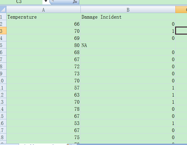
CSV保存
结构:第一列数值
第二列布尔值

# -*- coding: utf-8 -*-
"""
Created on Fri Jul 21 09:28:25 2017
@author: toby
CSV数据结构,第一列为数值,第二列为二分类型
"""
import csv
import numpy as np
import pandas as pd
from statsmodels.formula.api import glm
from statsmodels.genmod.families import Binomial
import matplotlib.pyplot as plt
import seaborn as sns
#该函数的其他的两个属性"notebook"和"paper"却不能正常显示中文
sns.set_context('poster')
fileName="challenger_data.csv"
reader = csv.reader(open(fileName))
#获取数据,类型:阵列
def getData():
'''Get the data '''
inFile = 'challenger_data.csv'
data = np.genfromtxt(inFile, skip_header=1, usecols=[1, 2],
missing_values='NA', delimiter=',')
# Eliminate NaNs 消除NaN数据
data = data[~np.isnan(data[:, 1])]
return data
def prepareForFit(inData):
''' Make the temperature-values unique, and count the number of failures and successes.
Returns a DataFrame'''
# Create a dataframe, with suitable columns for the fit
df = pd.DataFrame()
#np.unique返回去重的值
df['temp'] = np.unique(inData[:,0])
df['failed'] = 0
df['ok'] = 0
df['total'] = 0
df.index = df.temp.values
# Count the number of starts and failures
#inData.shape[0] 表示数据多少
for ii in range(inData.shape[0]):
#获取第一个值的温度
curTemp = inData[ii,0]
#获取第一个值的值,是否发生故障
curVal = inData[ii,1]
df.loc[curTemp,'total'] += 1
if curVal == 1:
df.loc[curTemp, 'failed'] += 1
else:
df.loc[curTemp, 'ok'] += 1
return df
#逻辑回归公式
def logistic(x, beta, alpha=0):
''' Logistic Function '''
#点积,比如np.dot([1,2,3],[4,5,6]) = 1*4 + 2*5 + 3*6 = 32
return 1.0 / (1.0 + np.exp(np.dot(beta, x) + alpha))
#不太懂
def setFonts(*options):
return
#绘图
def Plot(data,alpha,beta,picName):
#阵列,数值
array_values = data[:,0]
#阵列,二分类型
array_type = data[:,1]
plt.figure()
setFonts()
#改变指定主题的风格参数
sns.set_style('darkgrid')
#numpy输出精度局部控制
np.set_printoptions(precision=3, suppress=True)
plt.scatter(array_values, array_type, s=200, color="k", alpha=0.5)
#获取值列表
list_values = [row[1] for row in reader][1:]
list_values = [int(i) for i in list_values]
#获取列表最大值和最小值
max_value=max(list_values)
min_value=min(list_values)
#最大值和最小值留有多余空间
x = np.arange(min_value, max_value)
y = logistic(x, beta, alpha)
plt.hold(True)
plt.plot(x,y,'r')
#设置y轴坐标刻度
plt.yticks([0, 1])
#plt.xlim()返回当前的X轴绘图范围
plt.xlim([min_value,max_value])
outFile = picName
plt.ylabel("probability")
plt.xlabel("values")
plt.title("logistic regression")
#产生方格
plt.hold(True)
#图像外部边缘的调整
plt.tight_layout
plt.show(outFile)
#用于预测逻辑回归概率
def Prediction(x):
y = logistic(x, beta, alpha)
print("probability prediction:",y)
#获取数据
inData = getData()
#得到频率计算后的数据
dfFit = prepareForFit(inData)
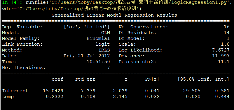
#Generalized Linear Model 建立二项式模型
model = glm('ok + failed ~ temp', data=dfFit, family=Binomial()).fit()
print(model.summary())
alpha = model.params[0]
beta = model.params[1]
Plot(inData,alpha,beta,"logiscti regression")
逻辑回归调参文档
默认参数
class sklearn.linear_model.LogisticRegression(penalty='l2', dual=False, tol=0.0001, C=1.0,fit_intercept=True, intercept_scaling=1, class_weight=None, random_state=None,solver='liblinear', max_iter=100, multi_class='ovr', verbose=0,warm_start=False, n_jobs=1)
乳腺癌逻辑回归调参测试脚本
# -*- coding: utf-8 -*-
"""
Created on Mon Jul 30 14:11:27 2018
@author: zhi.li04

官网调参文档
http://scikit-learn.org/stable/modules/generated/sklearn.linear_model.LogisticRegression.html

重要参数
penalty
在调参时如果我们主要的目的只是为了解决过拟合,一般penalty选择L2正则化就够了。但是如果选择L2正则化发现还是过拟合,即预测效果差的时候,就可以考虑L1正则化。另外,如果模型的特征非常多,我们希望一些不重要的特征系数归零,从而让模型系数稀疏化的话,也可以使用L1正则化。
tol:Tolerance for stopping criteria

n_jobs : int, default: 1
Number of CPU cores used when parallelizing over classes if multi_class=’ovr’”. This parameter is ignored when the ``solver``is set to ‘liblinear’ regardless of whether ‘multi_class’ is specified or not. If given a value of -1, all cores are used.
"""

from sklearn import metrics
import numpy as np
import matplotlib.pyplot as plt
from sklearn.linear_model import LogisticRegression
from sklearn.model_selection import train_test_split
from sklearn.datasets import load_breast_cancer


cancer=load_breast_cancer()
x_train,x_test,y_train,y_test=train_test_split(cancer.data,cancer.target,random_state=0)

#默认参数
logist=LogisticRegression()
logist.fit(x_train,y_train)

print("logistic regression with default parameters:")
print("accuracy on the training subset:{:.3f}".format(logist.score(x_train,y_train)))
print("accuracy on the test subset:{:.3f}".format(logist.score(x_test,y_test)))
print(logist.sparsify())
print("coefficience:")
print(logist.coef_)
print("intercept:")
print (logist.intercept_)
print()
'''
默认是l2惩罚
LogisticRegression(C=1.0, class_weight=None, dual=False, fit_intercept=True,
          intercept_scaling=1, max_iter=100, multi_class='ovr', n_jobs=1,
          penalty='l2', random_state=None, solver='liblinear', tol=0.0001,
          verbose=0, warm_start=False)
'''


#正则化l1
logist2=LogisticRegression(C=1,penalty='l1',tol=0.01)
logist2.fit(x_train,y_train)

print("logistic regression with pernalty l1:")
print("accuracy on the training subset:{:.3f}".format(logist2.score(x_train,y_train)))
print("accuracy on the test subset:{:.3f}".format(logist2.score(x_test,y_test)))
print("coefficience:")
print(logist2.coef_)
print("intercept:")
print (logist2.intercept_)
print()
'''
logistic regression:
accuracy on the training subset:0.955
accuracy on the test subset:0.958

logist.sparsify()
Out[6]:
LogisticRegression(C=1, class_weight=None, dual=False, fit_intercept=True,
          intercept_scaling=1, max_iter=100, multi_class='ovr', n_jobs=1,
          penalty='l1', random_state=None, solver='liblinear', tol=0.01,
          verbose=0, warm_start=False)

len(logist2.coef_[0])
Out[20]: 30
'''


#正则化l2
logist3=LogisticRegression(C=1,penalty='l2',tol=0.01)
logist3.fit(x_train,y_train)

print("logistic regression with pernalty l2:")
print("accuracy on the training subset:{:.3f}".format(logist3.score(x_train,y_train)))
print("accuracy on the test subset:{:.3f}".format(logist3.score(x_test,y_test)))
print("coefficience:")
print(logist3.coef_)
print("intercept:")
print (logist3.intercept_)
print()

- 正则化选择参数(惩罚项的种类)
penalty : str, ‘l1’or ‘l2’, default: ‘l2’
Usedto specify the norm used in the penalization. The ‘newton-cg’, ‘sag’ and‘lbfgs’ solvers support only l2 penalties.
- LogisticRegression默认带了正则化项。penalty参数可选择的值为"l1"和"l2".分别对应L1的正则化和L2的正则化,默认是L2的正则化。
- 在调参时如果我们主要的目的只是为了解决过拟合,一般penalty选择L2正则化就够了。但是如果选择L2正则化发现还是过拟合,即预测效果差的时候,就可以考虑L1正则化。另外,如果模型的特征非常多,我们希望一些不重要的特征系数归零,从而让模型系数稀疏化的话,也可以使用L1正则化。
- penalty参数的选择会影响我们损失函数优化算法的选择。即参数solver的选择,如果是L2正则化,那么4种可选的算法{‘newton-cg’, ‘lbfgs’, ‘liblinear’, ‘sag’}都可以选择。但是如果penalty是L1正则化的话,就只能选择‘liblinear’了。这是因为L1正则化的损失函数不是连续可导的,而{‘newton-cg’, ‘lbfgs’,‘sag’}这三种优化算法时都需要损失函数的一阶或者二阶连续导数。而‘liblinear’并没有这个依赖。
- dual : bool, default: False
Dualor primal formulation. Dual formulation is only implemented for l2 penalty withliblinear solver. Prefer dual=False whenn_samples > n_features.
- 对偶或者原始方法。Dual只适用于正则化相为l2 liblinear的情况,通常样本数大于特征数的情况下,默认为False。
- C : float, default: 1.0
Inverseof regularization strength; must be a positive float. Like in support vectormachines, smaller values specify stronger regularization.
- C为正则化系数λ的倒数,通常默认为1
- fit_intercept : bool, default: True
Specifiesif a constant (a.k.a. bias or intercept) should be added to the decisionfunction.
- 是否存在截距,默认存在
- intercept_scaling : float, default 1.
Usefulonly when the solver ‘liblinear’ is used and self.fit_intercept is set to True.In this case, x becomes [x, self.intercept_scaling], i.e. a “synthetic” featurewith constant value equal to intercept_scaling is appended to the instancevector. The intercept becomes intercept_scaling * synthetic_feature_weight.
Note!the synthetic feature weight is subject to l1/l2 regularization as all otherfeatures. To lessen the effect of regularization on synthetic feature weight(and therefore on the intercept) intercept_scaling has to be increased.
仅在正则化项为"liblinear",且fit_intercept设置为True时有用。
- 优化算法选择参数
solver
{‘newton-cg’, ‘lbfgs’, ‘liblinear’, ‘sag’}, default: ‘liblinear’
Algorithmto use in the optimization problem.
Forsmall datasets, ‘liblinear’ is a good choice, whereas ‘sag’ is
fasterfor large ones.
Formulticlass problems, only ‘newton-cg’, ‘sag’ and ‘lbfgs’ handle
multinomialloss; ‘liblinear’ is limited to one-versus-rest schemes.
‘newton-cg’,‘lbfgs’ and ‘sag’ only handle L2 penalty.
Notethat ‘sag’ fast convergence is only guaranteed on features with approximatelythe same scale. You can preprocess the data with a scaler fromsklearn.preprocessing.
Newin version 0.17: Stochastic Average Gradient descent solver.
- solver参数决定了我们对逻辑回归损失函数的优化方法,有四种算法可以选择,分别是:
a) liblinear:使用了开源的liblinear库实现,内部使用了坐标轴下降法来迭代优化损失函数。
b) lbfgs:拟牛顿法的一种,利用损失函数二阶导数矩阵即海森矩阵来迭代优化损失函数。
c) newton-cg:也是牛顿法家族的一种,利用损失函数二阶导数矩阵即海森矩阵来迭代优化损失函数。
d) sag:即随机平均梯度下降,是梯度下降法的变种,和普通梯度下降法的区别是每次迭代仅仅用一部分的样本来计算梯度,适合于样本数据多的时候。
- 从上面的描述可以看出,newton-cg, lbfgs和sag这三种优化算法时都需要损失函数的一阶或者二阶连续导数,因此不能用于没有连续导数的L1正则化,只能用于L2正则化。而liblinear通吃L1正则化和L2正则化。
- 同时,sag每次仅仅使用了部分样本进行梯度迭代,所以当样本量少的时候不要选择它,而如果样本量非常大,比如大于10万,sag是第一选择。但是sag不能用于L1正则化,所以当你有大量的样本,又需要L1正则化的话就要自己做取舍了。要么通过对样本采样来降低样本量,要么回到L2正则化。
- 从上面的描述,大家可能觉得,既然newton-cg, lbfgs和sag这么多限制,如果不是大样本,我们选择liblinear不就行了嘛!错,因为liblinear也有自己的弱点!我们知道,逻辑回归有二元逻辑回归和多元逻辑回归。对于多元逻辑回归常见的有one-vs-rest(OvR)和many-vs-many(MvM)两种。而MvM一般比OvR分类相对准确一些。郁闷的是liblinear只支持OvR,不支持MvM,这样如果我们需要相对精确的多元逻辑回归时,就不能选择liblinear了。也意味着如果我们需要相对精确的多元逻辑回归不能使用L1正则化了。
- 总结几种优化算法适用情况:
|
L1 |
liblinear |
liblinear适用于小数据集;如果选择L2正则化发现还是过拟合,即预测效果差的时候,就可以考虑L1正则化;如果模型的特征非常多,希望一些不重要的特征系数归零,从而让模型系数稀疏化的话,也可以使用L1正则化。 |
|
L2 |
liblinear |
libniear只支持多元逻辑回归的OvR,不支持MvM,但MVM相对精确。 |
|
L2 |
lbfgs/newton-cg/sag |
较大数据集,支持one-vs-rest(OvR)和many-vs-many(MvM)两种多元逻辑回归。 |
|
L2 |
sag |
如果样本量非常大,比如大于10万,sag是第一选择;但不能用于L1正则化。 |
具体OvR和MvM有什么不同下一节讲。
- 分类方式选择参数:
multi_class : str, {‘ovr’, ‘multinomial’}, default:‘ovr’
Multiclassoption can be either ‘ovr’ or ‘multinomial’. If the option chosen is ‘ovr’,then a binary problem is fit for each label. Else the loss minimised is themultinomial loss fit across the entire probability distribution. Works only forthe ‘newton-cg’, ‘sag’ and ‘lbfgs’ solver.
Newin version 0.18: Stochastic Average Gradient descent solver for ‘multinomial’case.
- ovr即前面提到的one-vs-rest(OvR),而multinomial即前面提到的many-vs-many(MvM)。如果是二元逻辑回归,ovr和multinomial并没有任何区别,区别主要在多元逻辑回归上。
- OvR和MvM有什么不同?
OvR的思想很简单,无论你是多少元逻辑回归,我们都可以看做二元逻辑回归。具体做法是,对于第K类的分类决策,我们把所有第K类的样本作为正例,除了第K类样本以外的所有样本都作为负例,然后在上面做二元逻辑回归,得到第K类的分类模型。其他类的分类模型获得以此类推。
而MvM则相对复杂,这里举MvM的特例one-vs-one(OvO)作讲解。如果模型有T类,我们每次在所有的T类样本里面选择两类样本出来,不妨记为T1类和T2类,把所有的输出为T1和T2的样本放在一起,把T1作为正例,T2作为负例,进行二元逻辑回归,得到模型参数。我们一共需要T(T-1)/2次分类。
可以看出OvR相对简单,但分类效果相对略差(这里指大多数样本分布情况,某些样本分布下OvR可能更好)。而MvM分类相对精确,但是分类速度没有OvR快。如果选择了ovr,则4种损失函数的优化方法liblinear,newton-cg,lbfgs和sag都可以选择。但是如果选择了multinomial,则只能选择newton-cg, lbfgs和sag了。
- 类型权重参数:(考虑误分类代价敏感、分类类型不平衡的问题)
class_weight : dictor ‘balanced’, default: None
Weightsassociated with classes in the form {class_label: weight}. If not given, allclasses are supposed to have weight one.
The“balanced” mode uses the values of y to automatically adjust weights inverselyproportional to class frequencies in the input data as n_samples / (n_classes *np.bincount(y)).
Notethat these weights will be multiplied with sample_weight (passed through thefit method) if sample_weight is specified.
Newin version 0.17: class_weight=’balanced’ instead of deprecatedclass_weight=’auto’.
- class_weight参数用于标示分类模型中各种类型的权重,可以不输入,即不考虑权重,或者说所有类型的权重一样。如果选择输入的话,可以选择balanced让类库自己计算类型权重,或者我们自己输入各个类型的权重,比如对于0,1的二元模型,我们可以定义class_weight={0:0.9, 1:0.1},这样类型0的权重为90%,而类型1的权重为10%。
- 如果class_weight选择balanced,那么类库会根据训练样本量来计算权重。某种类型样本量越多,则权重越低,样本量越少,则权重越高。当class_weight为balanced时,类权重计算方法如下:n_samples / (n_classes * np.bincount(y))
n_samples为样本数,n_classes为类别数量,np.bincount(y)会输出每个类的样本数,例如y=[1,0,0,1,1],则np.bincount(y)=[2,3]
- 那么class_weight有什么作用呢?
在分类模型中,我们经常会遇到两类问题:
第一种是误分类的代价很高。比如对合法用户和非法用户进行分类,将非法用户分类为合法用户的代价很高,我们宁愿将合法用户分类为非法用户,这时可以人工再甄别,但是却不愿将非法用户分类为合法用户。这时,我们可以适当提高非法用户的权重。
第二种是样本是高度失衡的,比如我们有合法用户和非法用户的二元样本数据10000条,里面合法用户有9995条,非法用户只有5条,如果我们不考虑权重,则我们可以将所有的测试集都预测为合法用户,这样预测准确率理论上有99.95%,但是却没有任何意义。这时,我们可以选择balanced,让类库自动提高非法用户样本的权重。
提高了某种分类的权重,相比不考虑权重,会有更多的样本分类划分到高权重的类别,从而可以解决上面两类问题。
当然,对于第二种样本失衡的情况,我们还可以考虑用下一节讲到的样本权重参数: sample_weight,而不使用class_weight。sample_weight在下一节讲。
- 样本权重参数:
sample_weight(fit函数参数)
- 当样本是高度失衡的,导致样本不是总体样本的无偏估计,从而可能导致我们的模型预测能力下降。遇到这种情况,我们可以通过调节样本权重来尝试解决这个问题。调节样本权重的方法有两种,第一种是在class_weight使用balanced。第二种是在调用fit函数时,通过sample_weight来自己调节每个样本权重。在scikit-learn做逻辑回归时,如果上面两种方法都用到了,那么样本的真正权重是class_weight*sample_weight.
- max_iter : int, default: 100
Usefulonly for the newton-cg, sag and lbfgs solvers. Maximum number of iterationstaken for the solvers to converge.
- 仅在正则化优化算法为newton-cg, sag and lbfgs 才有用,算法收敛的最大迭代次数。
- random_state : int seed, RandomState instance, default: None
The seed of the pseudo random number generator touse when shuffling the data. Used only in solvers ‘sag’ and ‘liblinear’.
- 随机数种子,默认为无,仅在正则化优化算法为sag,liblinear时有用。
- tol : float, default: 1e-4
Tolerance for stopping criteria.迭代终止判据的误差范围。
- verbose : int, default: 0
Forthe liblinear and lbfgs solvers set verbose to any positive number forverbosity.
- 日志冗长度int:冗长度;0:不输出训练过程;1:偶尔输出; >1:对每个子模型都输出
- warm_start : bool, default: False
Whenset to True, reuse the solution of the previous call to fit as initialization,otherwise, just erase the previous solution. Useless for liblinear solver.
Newin version 0.17: warm_start to support lbfgs, newton-cg, sag solvers.
- 是否热启动,如果是,则下一次训练是以追加树的形式进行(重新使用上一次的调用作为初始化),bool:热启动,False:默认值
- n_jobs : int, default: 1
Numberof CPU cores used during the cross-validation loop. If given a value of -1, allcores are used.
- 并行数,int:个数;-1:跟CPU核数一致;1:默认值
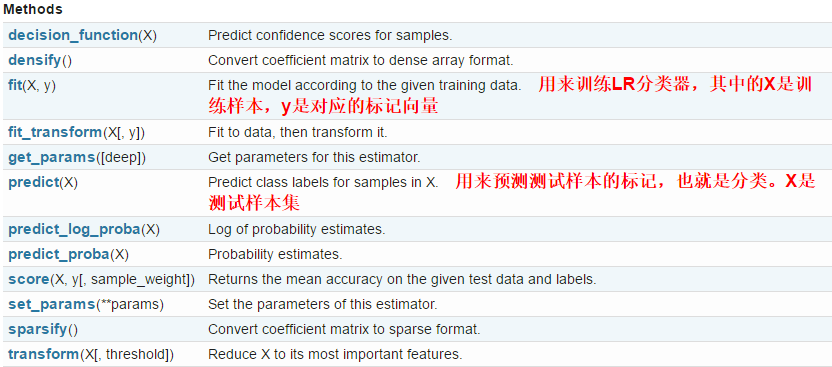
- LogisticRegression类中的方法
LogisticRegression类中的方法有如下几种,常用的是fit和predict
1 Logistic回归
假设现在有一些数据点,我们利用一条直线对这些点进行拟合(该线称为最佳拟合直线),这个拟合过程就称作为回归,如下图所示:
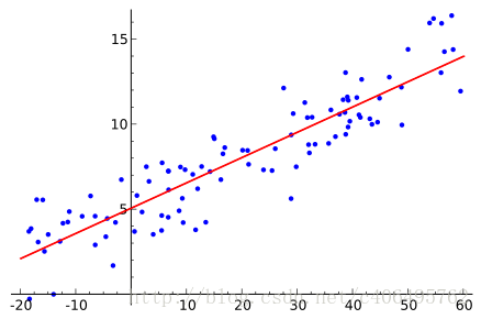
Logistic回归是回归的一种方法,它利用的是Sigmoid函数阈值在[0,1]这个特性。Logistic回归进行分类的主要思想是:根据现有数据对分类边界线建立回归公式,以此进行分类。其实,Logistic本质上是一个基于条件概率的判别模型(Discriminative Model)。
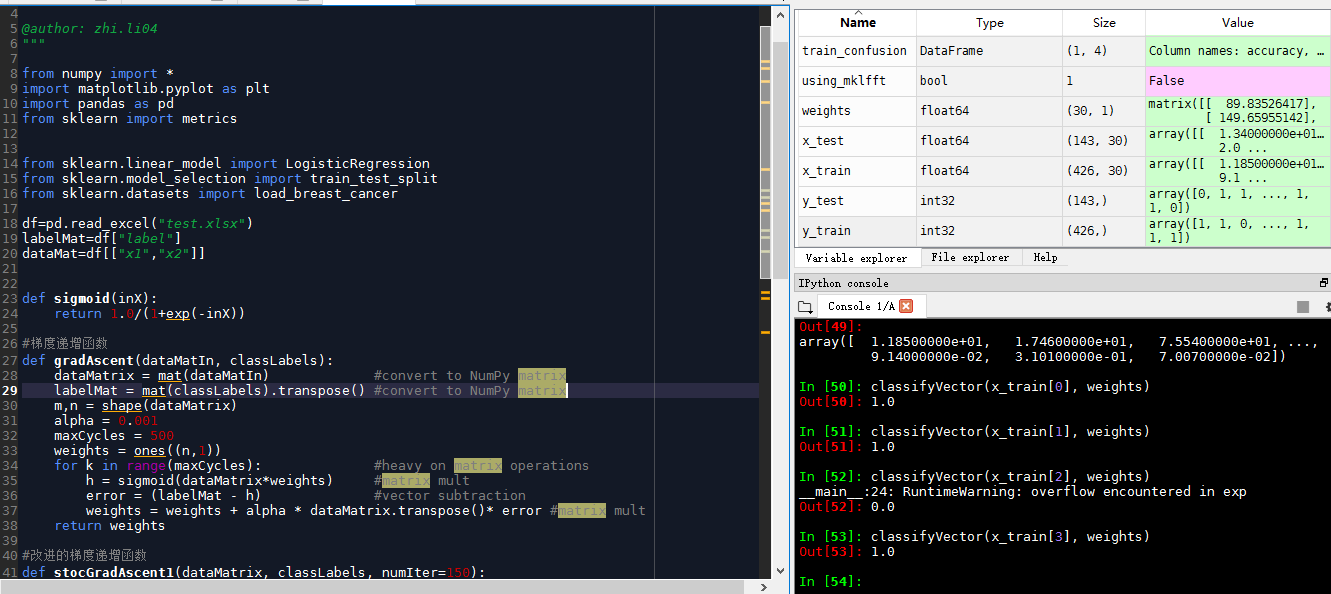
乳腺癌数据-逻辑回归源代码
算法思路:
sigmoid函数计算二分类概率
梯度上升法获取最优系数
随机梯度上升法获取最优系数,同时节约时间
# -*- coding: utf-8 -*-
"""
Created on Mon Jul 30 17:25:33 2018

@author: zhi.li04
"""

from numpy import *
import matplotlib.pyplot as plt
import pandas as pd
from sklearn import metrics


from sklearn.linear_model import LogisticRegression
from sklearn.model_selection import train_test_split
from sklearn.datasets import load_breast_cancer

df=pd.read_excel("test.xlsx")
labelMat=df["label"]
dataMat=df[["x1","x2"]]


def sigmoid(inX):
    return 1.0/(1+exp(-inX))

#梯度递增函数,返回最优系数
def gradAscent(dataMatIn, classLabels):
    dataMatrix = mat(dataMatIn)             #convert to NumPy matrix
    labelMat = mat(classLabels).transpose() #convert to NumPy matrix,transpose是置换
    m,n = shape(dataMatrix)                 #查看矩阵或者数组的维数
    alpha = 0.001
    maxCycles = 500
    weights = ones((n,1))
    for k in range(maxCycles):              #heavy on matrix operations
        h = sigmoid(dataMatrix*weights)     #matrix mult
        error = (labelMat - h)              #vector subtraction
        weights = weights + alpha * dataMatrix.transpose()* error #matrix mult
    return weights

#改进的梯度递增函数
def stocGradAscent1(dataMatrix, classLabels, numIter=150):
    m,n = shape(dataMatrix)
    weights = ones(n)   #initialize to all ones
    for j in range(numIter):
        dataIndex = range(m)
        for i in range(m):
            alpha = 4/(1.0+j+i)+0.0001    #apha decreases with iteration, does not
            randIndex = int(random.uniform(0,len(dataIndex)))#go to 0 because of the constant
            h = sigmoid(sum(dataMatrix[randIndex]*weights))
            error = classLabels[randIndex] - h
            weights = weights + alpha * error * dataMatrix[randIndex]
            #python3不支持,需要改进
            del(dataIndex[randIndex])
    return weights

def classifyVector(inX, weights):
    prob = sigmoid(sum(inX*weights))
    if prob > 0.5: return 1.0
    else: return 0.0

coef_matrix=gradAscent(dataMat, labelMat)

cancer=load_breast_cancer()
x_train,x_test,y_train,y_test=train_test_split(cancer.data,cancer.target,random_state=0)
weights=gradAscent(x_train, y_train)


predict=classifyVector(x_train[0], weights)
'''
exp(0)
Out[4]: 1.0

exp(1)
Out[5]: 2.7182818284590451

x = np.arange(4).reshape((2,2))

x
Out[24]:
array([[0, 1],
       [2, 3]])

np.transpose(x)
Out[25]:
array([[0, 2],
       [1, 3]])

classifyVector(x_train[0], weights)
Out[50]: 1.0

classifyVector(x_train[1], weights)
Out[51]: 1.0

classifyVector(x_train[2], weights)
__main__:24: RuntimeWarning: overflow encountered in exp
Out[52]: 0.0

classifyVector(x_train[3], weights)
Out[53]: 1.0
'''
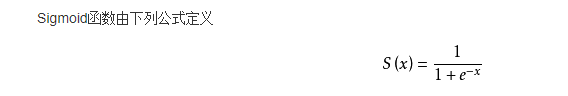
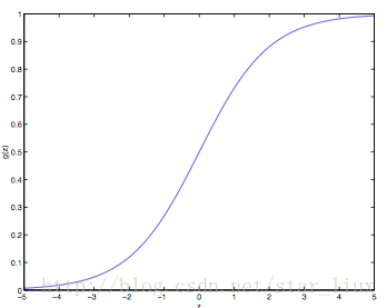
sigmoid函数
最早Logistic函数是皮埃尔·弗朗索瓦·韦吕勒在1844或1845年在研究它与人口增长的关系时命名的。广义Logistic曲线可以模仿一些情况人口增长(P)的 S 形曲线。起初阶段大致是指数增长;然后随着开始变得饱和,增加变慢;最后,达到成熟时增加停止。
Sigmoid函数是一个在生物学中常见的S型函数,也称为S型生长曲线。 [1] 在信息科学中,由于其单增以及反函数单增等性质,Sigmoid函数常被用作神经网络的阈值函数,将变量映射到0,1之间。
sigmoid公式
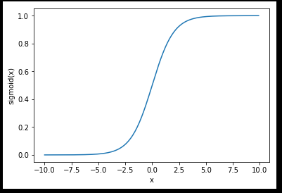
import sys
from pylab import*

t=arange(-10,10,0.1)
s=1/(1+exp(-t))

plot(t,s)
plt.xlabel("x")
plt.ylabel("sigmoid(x)")
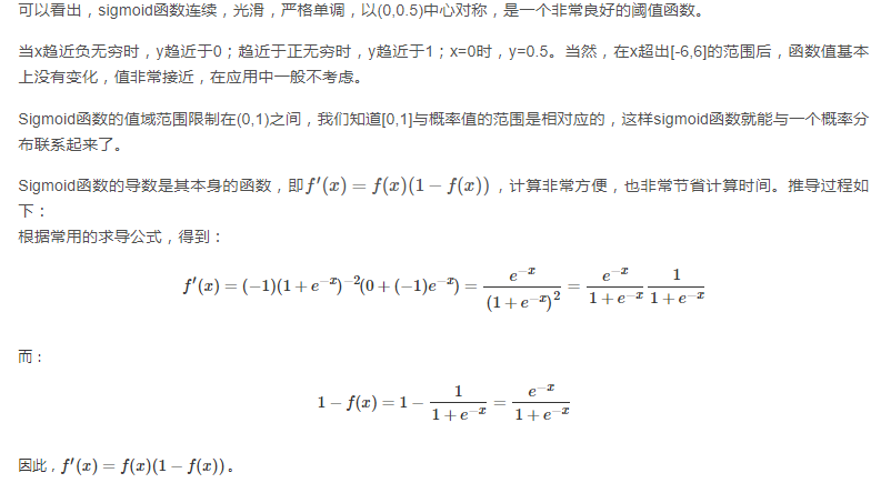
虽然sigmoid函数拥有良好的性质,可以用在分类问题上,如作为逻辑回归模型的分类器。但为什么偏偏选用这个函数呢?除了上述的数学上更易处理外,还有其本身的推导特性。
对于分类问题,尤其是二分类问题,都假定是服从伯努利分布。伯努利分布的概率质量函数PMF为:
机器学习中一个重要的预测模型逻辑回归(LR)就是基于Sigmoid函数实现的。LR模型的主要任务是给定一些历史的{X,Y},其中X是样本n个特征值,Y的取值是{0,1}代表正例与负例,通过对这些历史样本的学习,从而得到一个数学模型,给定一个新的X,能够预测出Y。LR模型是一个二分类模型,即对于一个X,预测其发生或不发生。但事实上,对于一个事件发生的情况,往往不能得到100%的预测,因此LR可以得到一个事件发生的可能性,超过50%则认为事件发生,低于50%则认为事件不发生
从LR的目的上来看,在选择函数时,有两个条件是必须要满足的:
1. 取值范围在0~1之间。
2. 对于一个事件发生情况,50%是其结果的分水岭,选择函数应该在0.5中心对称。
从这两个条件来看,Sigmoid很好的符合了LR的需求。关于逻辑回归的具体实现与相关问题,可看这篇文章Logistic函数(sigmoid函数) - wenjun’s blog,在此不再赘述。
用最大似然估计求逻辑回归参数
https://blog.csdn.net/star_liux/article/details/39666737
一.最大似然估计
选择一个(一组)参数使得实验结果具有最大概率。
A. 如果分布是离散型的,其分布律

设x1,x2,...xn是X1,X2,..Xn的一个样本值,则可知X1,..Xn取x1,..,x2的概率,即事件{X1 = x1,...,Xn=xn}发生的概率为:
这里,因为样本值是已知的,所以(2)是
最大似然估计:已知样本值x1,...xn,选取一组参数
B.如果分布X是连续型,其概率密度
设x1,..xn为相应X1,...Xn的一个样本值,则随机点(X1,...,Xn)落在(x1,..xn)的领域内的概率近似为:
最大似然估计即为求

C. 求最大似然估计参数的步骤:
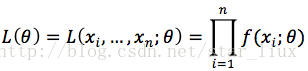
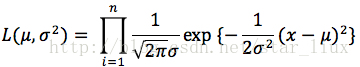
(1) 写出似然函数:
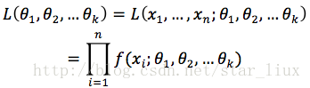
这里,n为样本数量,似然函数表示n个样本(事件)同时发生的概率。
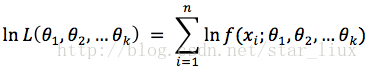
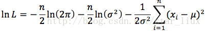
(2) 对似然函数取对数:
(3) 将对数似然函数对各参数求偏导数并令其为0,得到对数似然方程组。
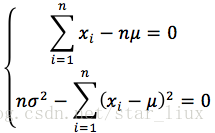
(4) 从方程组中解出各个参数。
D. 举例:
设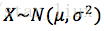

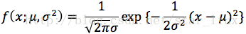
解:X的概率密度为:
似然函数为:
令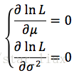
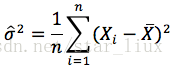
解得: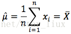
二.逻辑回归
逻辑回归不是回归,而是分类。是从线性回归中衍生出来的分类策略。当y值为只有两个值时(比如0,1),线性回归不能很好的拟合时,用逻辑回归来对其进行二值分类。
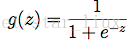
这里逻辑函数(S型函数)为:
于是,可得估计函数:
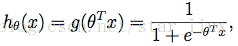
这里,我们的目的是求出一组
由于二值分类很像二项分布,我们把单一样本的类值假设为发生概率,则:
可以写成概率一般式:
由最大似然估计原理,我们可以通过m个训练样本值,来估计出
这里,
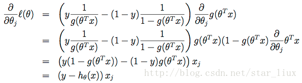
我们用随机梯度上升法,求使
这里
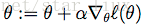
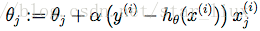
于是,随机梯度上升法迭代算法为:
repeat until convergence{
for i = 1 to m{
}
}
思考:
我们求最大似然函数参数的立足点是步骤C,即求出每个参数方向上的偏导数,并让偏导数为0,最后求解此方程组。由于
备注:
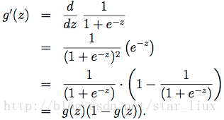
(a) 公式(14)的化简基于g(z)导函数,如下:
(b) 下图为逻辑函数g(z)的分布图:
https://blog.csdn.net/zjuPeco/article/details/77165974
前言
逻辑回归是分类当中极为常用的手段,因此,掌握其内在原理是非常必要的。我会争取在本文中尽可能简明地展现逻辑回归(logistic regression)的整个推导过程。
什么是逻辑回归
逻辑回归在某些书中也被称为对数几率回归,明明被叫做回归,却用在了分类问题上,我个人认为这是因为逻辑回归用了和回归类似的方法来解决了分类问题。
假设有一个二分类问题,输出为y∈{0,1}y∈{0,1},而线性回归模型产生的预测值为z=wTx+bz=wTx+b是实数值,我们希望有一个理想的阶跃函数来帮我们实现zz值到0/10/1值的转化。
然而该函数不连续,我们希望有一个单调可微的函数来供我们使用,于是便找到了Sigmoid functionSigmoid function来替代。
两者的图像如下图所示(图片出自文献2)
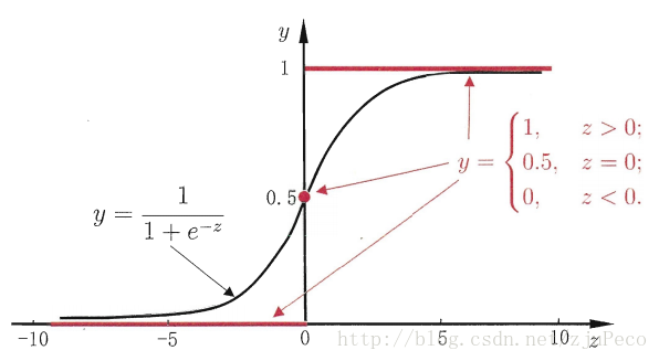
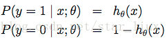
有了Sigmoid fuctionSigmoid fuction之后,由于其取值在[0,1][0,1],我们就可以将其视为类11的后验概率估计p(y=1|x)p(y=1|x)。说白了,就是如果有了一个测试点xx,那么就可以用Sigmoid fuctionSigmoid fuction算出来的结果来当做该点xx属于类别11的概率大小。
于是,非常自然地,我们把Sigmoid fuctionSigmoid fuction计算得到的值大于等于0.50.5的归为类别11,小于0.50.5的归为类别00。
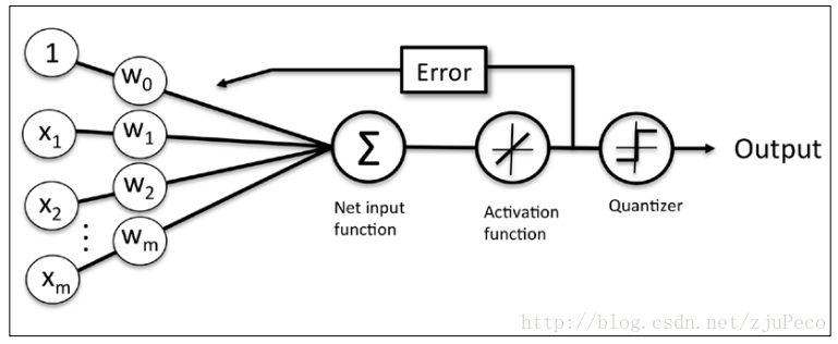
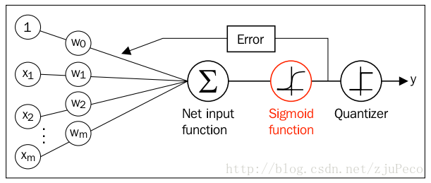
同时逻辑回归于自适应线性网络非常相似,两者的区别在于逻辑回归的激活函数时Sigmoid functionSigmoid function而自适应线性网络的激活函数是y=xy=x,两者的网络结构如下图所示(图片出自文献1)。
逻辑回归的代价函数
好了,所要用的几个函数我们都好了,接下来要做的就是根据给定的训练集,把参数ww给求出来了。要找参数ww,首先就是得把代价函数(cost function)给定义出来,也就是目标函数。
我们第一个想到的自然是模仿线性回归的做法,利用误差平方和来当代价函数。
其中,z(i)=wTx(i)+bz(i)=wTx(i)+b,ii表示第ii个样本点,y(i)y(i)表示第ii个样本的真实值,ϕ(z(i))ϕ(z(i))表示第ii个样本的预测值。
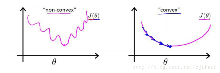
这时,如果我们将ϕ(z(i))=11+e−z(i)ϕ(z(i))=11+e−z(i)代入的话,会发现这时一个非凸函数,这就意味着代价函数有着许多的局部最小值,这不利于我们的求解。
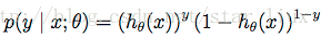
那么我们不妨来换一个思路解决这个问题。前面,我们提到了ϕ(z)ϕ(z)可以视为类11的后验估计,所以我们有
其中,p(y=1|x;w)p(y=1|x;w)表示给定ww,那么xx点y=1y=1的概率大小。
上面两式可以写成一般形式
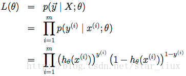
接下来我们就要用极大似然估计来根据给定的训练集估计出参数ww。
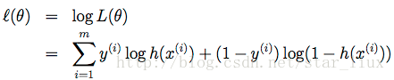
为了简化运算,我们对上面这个等式的两边都取一个对数
我们现在要求的是使得l(w)l(w)最大的ww。没错,我们的代价函数出现了,我们在l(w)l(w)前面加个负号不就变成就最小了吗?不就变成我们代价函数了吗?
为了更好地理解这个代价函数,我们不妨拿一个例子的来看看
也就是说
我们来看看这是一个怎么样的函数
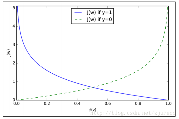
从图中不难看出,如果样本的值是11的话,估计值ϕ(z)ϕ(z)越接近11付出的代价就越小,反之越大;同理,如果样本的值是00的话,估计值ϕ(z)ϕ(z)越接近00付出的代价就越小,反之越大。
利用梯度下降法求参数
在开始梯度下降之前,要这里插一句,sigmoid functionsigmoid function有一个很好的性质就是
下面会用到这个性质。
还有,我们要明确一点,梯度的负方向就是代价函数下降最快的方向。什么?为什么?好,我来说明一下。借助于泰特展开,我们有
其中,f′(x)f′(x)和δδ为向量,那么这两者的内积就等于
当θ=πθ=π时,也就是δδ在f′(x)f′(x)的负方向上时,取得最小值,也就是下降的最快的方向了~
okay?好,坐稳了,我们要开始下降了。
没错,就是这么下降。没反应过来?那我再写详细一些
其中,wjwj表示第jj个特征的权重;ηη为学习率,用来控制步长。
重点来了。