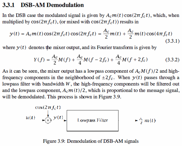
Demodulation of AM Signals
Demodulation is the process of extracting the message signal from the modulated signal.
The demodulation process depends on the type of modulation employed. For
DSB-AM and SSB-AM, the demodulation method is coherent demodulation, which
requires the existence of a signal with the same frequency and phase of the carrier at
the receiver. For conventional AM, envelope detectors are used for demodulation. In
this case precise knowledge of the frequency and the phase of the carrier at the receiver
is not crucial, so the demodulation process is much easier. Coherent demodulation for
DSB-AM and SSB-AM consists of multiplying (mixing) the modulated signal by a sinusoidal
with the same frequency and phase of the carrier and then passing the product
through a lowpass filter. The oscillator that generates the required sinusoidal at the
receiver is called the local oscillator.
Matlab Coding

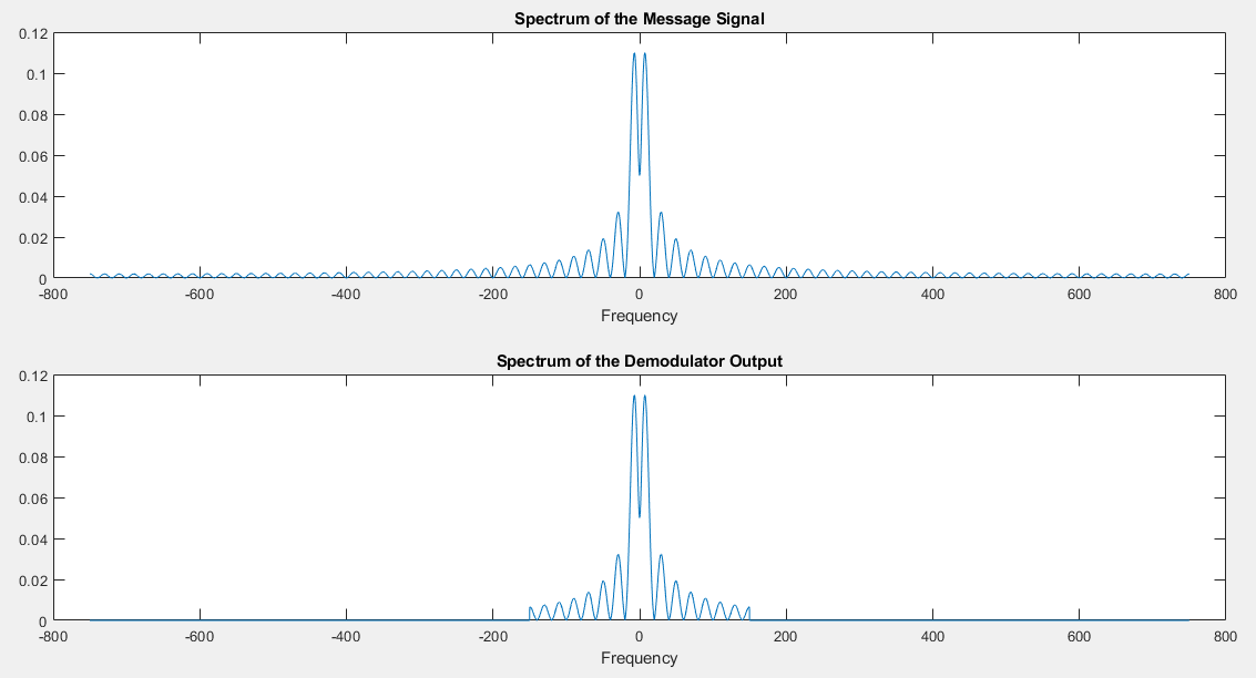
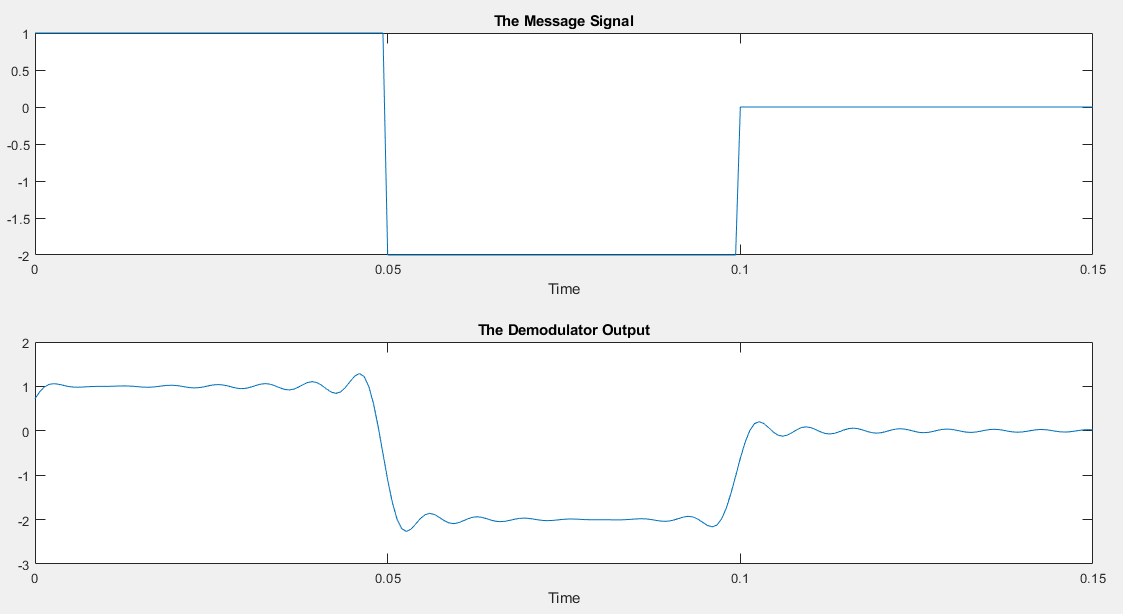
1 % MATLAB script for Illustrative Problem 3.5.
 2 % Demonstration script for DSB-AM demodulation. The message signal
 3 % is +1 for 0 < t < t0/3, -2 for t0/3 < t < 2t0/3, and zero otherwise.
 4 echo on
 5 t0=.15;                                 % signal duration
 6 ts=1/1500;                              % sampling interval
 7 fc=250;                                 % carrier frequency
 8 fs=1/ts;                                % sampling frequency
 9 t=[0:ts:t0];                            % time vector
10 df=0.3;                                 % desired frequency resolution
11 % message signal
12 m=[ones(1,t0/(3*ts)),-2*ones(1,t0/(3*ts)),zeros(1,t0/(3*ts)+1)];
13 c=cos(2*pi*fc.*t);                      % carrier signal
14 u=m.*c;                                 % modulated signal
15 y=u.*c;                             % mixing
16 [M,m,df1]=fftseq(m,ts,df);              % Fourier transform
17 M=M/fs;                                 % scaling
18 [U,u,df1]=fftseq(u,ts,df);              % Fourier transform
19 U=U/fs;                                 % scaling
20 [Y,y,df1]=fftseq(y,ts,df);              % Fourier transform
21 Y=Y/fs;                                 % scaling
22 f_cutoff=150;                           % cutoff freq. of the filter
23 n_cutoff=floor(150/df1);                % Design the filter.
24 f=[0:df1:df1*(length(y)-1)]-fs/2;
25 H=zeros(size(f));
26 H(1:n_cutoff)=2*ones(1,n_cutoff);
27 H(length(f)-n_cutoff+1:length(f))=2*ones(1,n_cutoff);
28 DEM=H.*Y;                           % spectrum of the filter output
29 dem=real(ifft(DEM))*fs;             % filter output
30 pause % Press a key to see the effect of mixing.
31 clf
32 subplot(3,1,1)
33 plot(f,fftshift(abs(M)))
34 title('Spectrum of the Message Signal')
35 xlabel('Frequency')
36 subplot(3,1,2)
37 plot(f,fftshift(abs(U)))
38 title('Spectrum of the Modulated Signal')
39 xlabel('Frequency')
40 subplot(3,1,3)
41 plot(f,fftshift(abs(Y)))
42 title('Spectrum of the Mixer Output')
43 xlabel('Frequency')
44 pause % Press a key to see the effect of filtering on the mixer output.
45 clf
46 subplot(3,1,1)
47 plot(f,fftshift(abs(Y)))
48 title('Spectrum of the Mixer Output')
49 xlabel('Frequency')
50 subplot(3,1,2)
51 plot(f,fftshift(abs(H)))
52 title('Lowpass Filter Characteristics')
53 xlabel('Frequency')
54 subplot(3,1,3)
55 plot(f,fftshift(abs(DEM)))
56 title('Spectrum of the Demodulator output')
57 xlabel('Frequency')
58 pause % Press a key to compare the spectra of the message and the received signal.
59 clf
60 subplot(2,1,1)
61 plot(f,fftshift(abs(M)))
62 title('Spectrum of the Message Signal')
63 xlabel('Frequency')
64 subplot(2,1,2)
65 plot(f,fftshift(abs(DEM)))
66 title('Spectrum of the Demodulator Output')
67 xlabel('Frequency')
68 pause % Press a key to see the message and the demodulator output signals.
69 subplot(2,1,1)
70 plot(t,m(1:length(t)))
71 title('The Message Signal')
72 xlabel('Time')
73 subplot(2,1,2)
74 plot(t,dem(1:length(t)))
75 title('The Demodulator Output')
76 xlabel('Time')


The effect of mixing

The effect of filtering on the mixer output
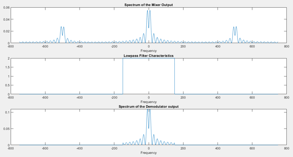
Compare the spectra of the message and the received signal
The message and the demodulator output signals
Reference,
1. <<Contemporary Communication System using MATLAB>> - John G. Proakis