Keras（三）backend 兼容 Regressor 回归 Classifier 分类 原理及实例

原文链接：http://www.one2know.cn/keras4/

backend 兼容

• backend，即基于什么来做运算
  Keras 可以基于两个Backend，一个是 Theano，一个是 Tensorflow
• 查看当前backend
  import keras
  输出：
  Using Theano Backend.
  或者
  Using TensorFlow backend.
• 修改backend
  找到~/.keras/keras.json文件，在文件内修改，每次import的时候，keras就会检查这个文件

{   # 后端为theano
	"image_dim_ordering": "tf",
	"epsilon": 1e-07,
	"floatx": "float32",
	"backend": "theano"
}
{   # 后端为tensorflow
	"image_dim_ordering": "tf",
	"epsilon": 1e-07,
	"floatx": "float32",
	"backend": "tensorflow"
}

但这样修改后，import的时候会出现错误信息，可以在terminal中直接输入临时环境变量执行：
KERAS_BACKEND=tensorflow python3 -c "from keras import backend"
最好是在python代码中import keras前加入一个环境变量修改的语句，这种方法仅在这个脚本生效：
import os
os.environ['KERAS_BACKEND']='theano' # os.environ['KERAS_BACKEND']='tensorflow'

Regressor 回归

• 神经网络可以用来模拟回归问题，给出一组数据，用一条线来对数据进行拟合，并可以预测新输入 x 的输出值
• 导入模块并创建数据
  models.Sequential 用来一层一层的去建立神经层
  layers.Dense 意思是这个神经层是全连接层

import numpy as np
np.random.seed(1)
from keras.models import Sequential
from keras.layers import Dense
import matplotlib.pyplot as plt

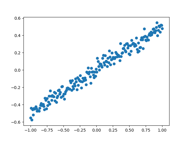
# 创建一组数据
x = np.linspace(-1,1,200)
np.random.shuffle(x)
y = 0.5 * x + np.random.normal(0,0.05,(200,))
plt.scatter(x,y)
plt.show()

x_train,y_train = x[:160],y[:160]
x_test,y_test = x[160:],y[160:]

输出：

• 建立模型
  用 Sequential 建立 model，再用model.add添加神经层，添加的是Dense全连接神经层
  参数有两个，一个是输入数据和输出数据的维度，本代码的例子中 x 和 y 是一维的

model = Sequential()
model.add(Dense(input_dim=1,output_dim=1))

• 激活模型
  参数中，误差函数loss用的是mse均方误差；优化器optimizer用的是sgd随机梯度下降法

model.compile(loss='mse', optimizer='sgd')

• 训练模型
  训练的时候用 model.train_on_batch 一批一批的训练 x_train, y_train。默认的返回值是cost，每100步输出一下结果

print('Training -------------')
for step in range(301):
    cost = model.train_on_batch(x_train,y_train) # 返回训练损失
    if step % 100 == 0:
        print('train cost',cost)

输出：

train cost 0.39069265
train cost 0.10105395
train cost 0.027371023
train cost 0.008624705

• 检验模型
  用到的函数是 model.evaluate，输入测试集的x和y， 输出 cost，weights 和 biases。其中 weights 和 biases 是取在模型的第一层 model.layers[0] 学习到的参数（一共就一层）

print('
Testing ------------')
cost = model.evaluate(x_test, y_test, batch_size=40)
print('test cost:', cost)
W, b = model.layers[0].get_weights()
print('Weights=', W, '
biases=', b)

输出：

Testing ------------
40/40 [==============================] - 0s 900us/step
test cost: 0.011580094695091248
Weights= [[0.64299107]] 
biases= [0.00309446]

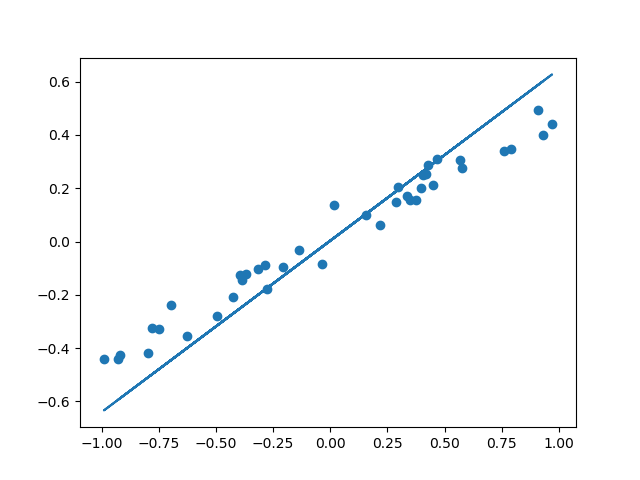
• 可视化结果

y_pred = model.predict(x_test)
plt.scatter(x_test, y_test)
plt.plot(x_test, y_pred)
plt.show()

输出：

• 整体代码

import numpy as np
np.random.seed(1)
from keras.models import Sequential
from keras.layers import Dense
import matplotlib.pyplot as plt

# 创建一组数据
x = np.linspace(-1,1,200)
np.random.shuffle(x)
y = 0.5 * x + np.random.normal(0,0.05,(200,))
plt.scatter(x,y)
plt.show()

x_train,y_train = x[:160],y[:160]
x_test,y_test = x[160:],y[160:]

model = Sequential()
model.add(Dense(input_dim=1,output_dim=1))

model.compile(loss='mse', optimizer='sgd')

# 分批训练模型
print('Training -------------')
for step in range(301):
    cost = model.train_on_batch(x_train,y_train) # 返回训练损失
    if step % 100 == 0:
        print('train cost',cost)

# 测速
print('
Testing ------------')
cost = model.evaluate(x_test, y_test, batch_size=40)
print('test cost:', cost)
W, b = model.layers[0].get_weights()
print('Weights=', W, '
biases=', b)

# 可视化
y_pred = model.predict(x_test)
plt.scatter(x_test, y_test)
plt.plot(x_test, y_pred)
plt.show()

Classifier 分类

• 以数据集MNIST构建一个分类神经网路
• 数据预处理
  Keras 自身就有 MNIST 这个数据包，再分成训练集和测试集。x 是一张张图片，y 是每张图片对应的标签，即它是哪个数字。
  输入的 x 变成 60,000×784(28x28的矩阵) 的数据，然后除以 255 进行标准化，因为每个像素都是在 0 到 255 之间的，标准化之后就变成了 0 到 1 之间。
  对于 y，要用到 Keras 改造的 numpy 的一个函数 np_utils.to_categorical，把 y 变成了 one-hot 的形式，即之前 y 是一个数值， 在 0-9 之间，现在是一个大小为 10 的向量，它属于哪个数字，就在哪个位置为 1，其他位置都是 0。

from keras.datasets import mnist
from keras.utils import np_utils
(x_train,y_train),(x_test,y_test) = mnist.load_data()

x_train = x_train.reshape(x_train.shape[0],-1)/255 # 标准化
x_test = x_test.reshape(x_test.shape[0],-1)/255
y_train = np_utils.to_categorical(y_train,num_classes=10)
y_test = np_utils.to_categorical(y_test,num_classes=10)

print(x_train[0].shape)
print(y_train[:3])

输出：

(784,)
[[0. 0. 0. 0. 0. 1. 0. 0. 0. 0.]
 [1. 0. 0. 0. 0. 0. 0. 0. 0. 0.]
 [0. 0. 0. 0. 1. 0. 0. 0. 0. 0.]]

• 建立神经网路
  相关的包：
  models.Sequential 用来一层一层一层的去建立神经层
  layers.Dense 意思是这个神经层是全连接层
  layers.Activation 激励函数
  optimizers.RMSprop 优化器采用 RMSprop，加速神经网络训练方法
• 建立模型
  在回归网络中用到的是 model.add 一层一层添加神经层，今天的方法是直接在模型的里面加多个神经层。好比一个水管，一段一段的，数据是从上面一段掉到下面一段，再掉到下面一段
  第一段就是加入 Dense 神经层。32 是输出的维度，784 是输入的维度。 第一层传出的数据有 32 个 feature，传给激励单元，激励函数用到的是 relu 函数。 经过激励函数之后，就变成了非线性的数据。 然后再把这个数据传给下一个神经层，这个 Dense 我们定义它有 10 个输出的 feature。同样的，此处不需要再定义输入的维度，因为它接收的是上一层的输出。 接下来再输入给下面的 softmax 函数，用来分类
  接下来用 RMSprop 作为优化器，它的参数包括学习率等，可以通过修改这些参数来看一下模型的效果

import numpy as np
np.random.seed(1)
from keras.models import Sequential
from keras.layers import Dense,Activation
from keras.optimizers import RMSprop

model = Sequential([
    Dense(32,input_dim=784),
    Activation('relu'),
    Dense(10),
    Activation('softmax')
])

# 优化器
rmsprop = RMSprop(lr=0.001,rho=0.9,epsilon=1e-08,decay=0.0)

# 激活模型
model.compile(optimizer=rmsprop,loss='categorical_crossentropy',metrics=['accuracy'])

• 训练网络
  这里用到的是 fit 函数，把训练集的 x 和 y 传入之后，nb_epoch 表示把整个数据训练多少次，batch_size 每批处理32个

print('Training --------------')
model.fit(x_train,y_train,epochs=2,batch_size=32)

• 测试模型
  接下来就是用测试集来检验一下模型，方法和回归网络中是一样的，运行代码之后，可以输出 accuracy 和 loss。

print('
Testing --------------')
loss,accuracy = model.evaluate(x_test,y_test)
print('test loss:',loss)
print('test accuracy:',accuracy)

输出：

test loss: 0.19889679334759713
test accuracy: 0.9396

• 完整代码

from keras.datasets import mnist
from keras.utils import np_utils
from keras.models import Sequential
from keras.layers import Dense,Activation
from keras.optimizers import RMSprop
(x_train,y_train),(x_test,y_test) = mnist.load_data()

x_train = x_train.reshape(x_train.shape[0],-1)/255 # 标准化
x_test = x_test.reshape(x_test.shape[0],-1)/255
y_train = np_utils.to_categorical(y_train,num_classes=10)
y_test = np_utils.to_categorical(y_test,num_classes=10)

print(x_train[0].shape)
print(y_train[:3])

# 创建模型
model = Sequential([
    Dense(32,input_dim=784),Activation('relu'),
    Dense(10),Activation('softmax'),
])

# 优化器
rmsprop = RMSprop(lr=0.001,rho=0.9,epsilon=1e-08,decay=0.0)

# 激活模型
model.compile(optimizer=rmsprop,loss='categorical_crossentropy',metrics=['accuracy'])

# 训练
print('Training --------------')
model.fit(x_train,y_train,epochs=2,batch_size=32)

# 测试
print('
Testing --------------')
loss,accuracy = model.evaluate(x_test,y_test)
print('test loss:',loss)
print('test accuracy:',accuracy)