Depth-first search
Depth-first search (DFS) is an algorithm for traversing or searching tree or graph data structures.
The algorithm starts at the root node (selecting some arbitrary node as the root node in the case of a graph) and explores as far as possible along each branch before backtracking 回溯.
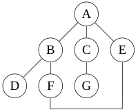
For the following graph:
a depth-first search starting at A,
assuming that the left edges in the shown graph are chosen before right edges,
and assuming the search remembers previously visited nodes and will not repeat them (since this is a small graph),
will visit the nodes in the following order: A, B, D, F, E, C, G.
The edges traversed in this search form a Trémaux tree, a structure with important applications in graph theory.
Performing the same search without remembering previously visited nodes results in visiting nodes in the order A, B, D, F, E, A, B, D, F, E, etc. forever, caught in the A, B, D, F, E cycle and never reaching C or G.
Iterative deepening is one technique to avoid this infinite loop and would reach all nodes.
深度优先的算法实现
Input: A graph G and a vertex v of G
Output: All vertices reachable from v labeled as discovered
A recursive implementation of DFS:[5]
1  procedure DFS(G,v):
2      label v as discovered
3      for all edges from v to w in G.adjacentEdges(v) do
4          if vertex w is not labeled as discovered then
5              recursively call DFS(G,w)
The order in which the vertices are discovered by this algorithm is called the lexicographic order.
A non-recursive implementation of DFS with worst-case space complexity O(|E|):[6] (使用栈,先进后出)
1  procedure DFS-iterative(G,v):
2      let S be a stack
3      S.push(v)
4      while S is not empty
5          v = S.pop()
6          if v is not labeled as discovered:
7              label v as discovered
8              for all edges from v to w in G.adjacentEdges(v) do
9                  S.push(w)
These two variations of DFS visit the neighbors of each vertex in the opposite order from each other: the first neighbor of v visited by the recursive variation is the first one in the list of adjacent edges, while in the iterative variation the first visited neighbor is the last one in the list of adjacent edges. The recursive implementation will visit the nodes from the example graph in the following order: A, B, D, F, E, C, G. The non-recursive implementation will visit the nodes as: A, E, F, B, D, C, G.
The non-recursive implementation is similar to breadth-first search but differs from it in two ways:
- it uses a stack instead of a queue, and
- it delays checking whether a vertex has been discovered until the vertex is popped from the stack rather than making this check before adding the vertex.
Breadth-first search
Breadth-first search (BFS) is an algorithm for traversing or searching tree or graph data structures.
It starts at the tree root (or some arbitrary node of a graph, sometimes referred to as a 'search key'[1]), and explores all of the neighbor nodes at the present depth prior to moving on to the nodes at the next depth level.
It uses the opposite strategy as depth-first search, which instead explores the highest-depth nodes first before being forced to backtrack回溯 and expand shallower nodes.
shallower是shallow的比较级,较浅的
广度优先的实现 (使用队列,先进先出)
Input: A graph Graph and a starting vertex顶点 root of Graph
Output: Goal state. The parent links trace the shortest path back to root
1  procedure BFS(G,start_v):
2      let S be a queue
3      S.enqueue(start_v)
4      while S is not empty
5          v = S.dequeue()
6          if v is the goal:
7              return v
8          for all edges from v to w in G.adjacentEdges(v) do
9              if w is not labeled as discovered:
10                 label w as discovered
11                 w.parent = v
12                 S.enqueue(w)
More details
This non-recursive implementation is similar to the non-recursive implementation of depth-first search, but differs from it in two ways:
- it uses a queue (First In First Out) instead of a stack and
- it checks whether a vertex顶点 has been discovered before enqueueing the vertex rather than delaying this check until the vertex is dequeued from the queue.
The Q queue contains the frontier along which the algorithm is currently searching.
Nodes can be labelled as discovered by storing them in a set, or by an attribute on each node, depending on the implementation.
Note that the word node is usually interchangeable with the word vertex.
The parent attribute of each vertex is useful for accessing the nodes in a shortest path, for example by backtracking from the destination node up to the starting node, once the BFS has been run, and the predecessors nodes have been set.
Breadth-first search produces a so-called breadth first tree. You can see how a breadth first tree looks in the following example.
